Reaching Equilibrium
At the end of setting up initial conditions, at the end of the model, and perhaps during
multiple intermediate stages, the model must reach “equilibrium.” In the examples so far, this
is done with the simple command model solve. But how do you know when you have reached
equilibrium? How can you tell if you have performed more cycles than is necessary, or if some
specific part of the model still needs computation time?
Calculation cycles in FLAC3D can be performed manually with the model step or
model cycle command. There are occasions where this is useful, most often when you have
prescribed a velocity at a boundary and want to step until a specific total displacement has
been reached. Generally, however, you wish to cycle until a certain condition has been
reached—for example, a dynamic simulation could cycle until a certain amount of time has passed.
The model solve command allows cycling to continue until one or more limits (specified
using subsequent keywords) has been met. In a static model, the most common limit of interest
is “until the model is in equilibrium.”
Because FLAC3D uses an iterative procedure informed by physics to reach static equilibrium, when we refer to being “in equilibrium,” we mean the same thing as being fully converged to a static solution. FLAC3D provides a number of different ways to measure and visualize how close you are to being converged or having reached an equilibrium state in your model. But, as always, the more you are aware of the issues involved, the more efficient and accurate your models are likely to be.
Convergence Criteria
FLAC3D has five different criteria available to determine when equilibrium is reached. Maximum Out-of-Balance Force, Local Force Ratio, Average Force Ratio, Maximum Force Ratio, and Convergence. Each of these options is described below (see Out-of-Balance Force and Ratio Calculation for more detailed formula).
Maximum Out-of-Balance Force
The first and simplest measure used for convergence is called the maximum out-of-balance force. While no longer used often, it is still available both as a
model solvecriteria and to thezone.unbalFISH intrinsic.Every gridpoint (or structural node) in the model receives forces from zones, elements, gravity, etc. Each of these forces is added together, resulting in the net forces acting on a gridpoint. The maximum out-of-balance force is the maximum absolute value of any one component of the force remaining after all forces are summed together. This is the force that drives the gridpoint in the direction of equilibrium. If the force is zero, the gridpoint can be thought of as being converged, or at equilibrium.
As a measure of overall convergence, the major drawback of maximum out-of-balance force is that it is not a unitless measure. The appropriate target value is dependent on the model size, zone size, material properties, and stress magnitude. It is impossible to provide a single value to use as a rule of thumb. This is why it is no longer in common use as a solve criteria.
Local Maximum Force Ratio
The local force ratio is a unitless measure of local convergence at a gridpoint. The idea is simple: divide the out-of-balance component remaining after summing forces by a measure of the total forces being applied to the gridpoint. For performance purposes, we use the “Manhattan norm” or “Taxicab norm” of a vector, defined as:
\[\langle v_i \rangle = |v_x| + |v_y| + |v_z|\]or the sum of the absolute values of the components of the vector. The local force ratio can then be defined as:
\[\frac{\langle \sum_i f_i\rangle}{\sum_i \langle f_i \rangle}\]where \(f_i\) are all the force vectors being added to a gridpoint.
The local maximum force ratio is the maximum local ratio of any gridpoint in the model. This is a very conservative measure of the convergence of a model. However it has a weakness when there is less than two forces being applied to a gridpoint, or when all forces being applied to a gridpoint act in the same direction. In this circumstance, the only “equilibrium” value possible is for both numerator and denominator to converge toward zero; the ratio between them will tend toward 1.
FLAC3D will detect when only one force vector is being applied to a gridpoint and automatically remove it from consideration. But if multiple aligned forces are acting on a gridpoint, or if the second force is negligible compared to a main driving force, then this check is insufficient. These points will dominate the maximum local force ratio, and the model will seem to never effectively converge.
In practice this does not happen very often. The majority of models never see this effect. But it does happen, and so maximum local force ratio is not used as the default convergence criteria for
model solvein order to guarantee that any given model will converge using the default criteria.The last local force ratio calculated for a gridpoint is stored and is available to FISH as
gp.ratioand to plot items as the Local Force Ratio.
Average Force Ratio
The average force ratio is defined as the sum of all out-of-balance force components at every gridpoint divided by the sum of all total forces applied at a gridpoint. Or:
\[\frac{ \sum_j^n \langle \sum_i f_i \rangle }{ \sum_j^n \sum_i \langle f_i \rangle }\]This measure serves as a reliable measure of the overall convergence of the system. For models that are relatively uniform, it performs very well. It is bulletproof enough that the default convergence criteria for
model solveis ratio-average 1e-5.However, for very non-uniform models, the effects of localized convergence problems can be lost in the average, making the user unaware that an area that might be of most interest still needs computation. This can occur either because of disparities in zone size, or because of large differences in stiffness. For large complex models, this measure should be checked carefully before being trusted. See the following discussion.
Maximum Force Ratio
The maximum force ratio is defined as the maximum out-of-balance force divided by the average total force acting on all gridpoints. The average total force is defined as:
\[\frac{\sum_j^n \sum_i \langle f_i^j \rangle}{N}\]where \(N\) is the total number of gridpoints in the model.
Convergence
The convergence solve was created as a means of giving the user more control over the convergence criteria desired and overcoming the possible disadvantages of relying on the local force ratio.
First - a new gridpoint field variable called the Local Force Target is created. This value defaults to 1e-4 in every gridpoint and node. It can be changed with the
zone gridpoint initialize ratio-targetcommand and with thegp.ratio.targetFISH intrinsic. This value indicates the local force ratio that is to be considered “converged” for that specific gridpoint. This means that the local convergence criteria can vary in different locations of the grid.We define a new quantity, unimaginatively called the convergence, that is the ratio of the current local force ratio to the target local force ratio. A convergence of 1.0 is therefore considered “converged”. The maximum convergence is then a measure of overall model convergence tied to the convergence keyword in
model solve. The convergence value is available to plot items, and to FISH as thegp.convergenceintrinsic. By default, a convergence of 1.0 is exactly the same as a ratio-local limit of 1e-4.In the event that the local ratio calculation is failing in corner cases, the ratio-target can be set to a high value in that gridpoint or node, effectively removing them from the overall convergence criteria. In addition, it is not unusual for a small region of the model to have an overly large effect on the time it takes to reach convergence—either because they are very small, or because they are very stiff, or both. For example, it is not unusual for a small number of very stiff structural supports to dominate the convergence time of a very large model. The ratio-target for those nodes could be set to 1e-3 or even higher, relaxing the criteria for those nodes once it is determined that this will have negligible effect on the model results of primary interest.
Ratio
The four convergence measures local ratio, maximum ratio, average ratio, and convergence can be referred by the single ratio keyword. By default, ratio maps to the average force ratio. The
zone ratiocommand can be used to indicate that ratio should mean local ratio, maximum ratio, or convergence instead. This allows the user to choose which criteria is driving various servo-driven capabilities of the code that are tied to the ratio value.Note that in order for default servo settings to remain generally valid the value of some convergence measures are scaled to bring them into the expected range for the default average ratio criteria. ratio-local and ratio-maximum are multiplied by 0.1, and convergence is multiplied by 1e-5.
In many cases, you can also explicitly indicate which criteria you mean by using the ratio-average, ratio-local, ratio-maximum, or convergence keywords.
Choosing Convergence Criteria
The default convergence criteria if none is specified for a model solve command is a ratio of 1e-5. In our experience, an average force ratio of 1e-5 corresponds to a local force ratio limit of around 1e-4 for a model of average complexity. This is why 1e-4 was chosen as a default ratio-target.
A maximum local ratio of 1e-4 is generally sufficient, even conservative, for most engineering applications. A maximum local ratio of 1e-3, or even as high as 1e-2 may be sufficient for many purposes. This is especially true for intermediate stages (excavation sequences, etc.) of a model, where taking the time to reach “full” convergence after every step may have negligible effects on the final state of a model.
- In general, we recommend that you use the
zone ratioandstructure ratiocommands to set the default criterial to convergence at the start of every data file. You can also explicitly use a convergence of 1 based on a ratio-target of 1e-4. If computation time is limited you can consider raising the default convergence value. Whether or not these target convergence criteria are raised, we recommend you take the time to evaluate the model to ensure that you have sufficient convergence for the results you are interested in. This is discussed in the next section.
Evaluating Equilibrium
For the purposes of illustration, we will demonstrate with a cartoonishly simple model of a surface excavation surrounded by a reinforcing wall. The basic geometry is shown in Figure 1.
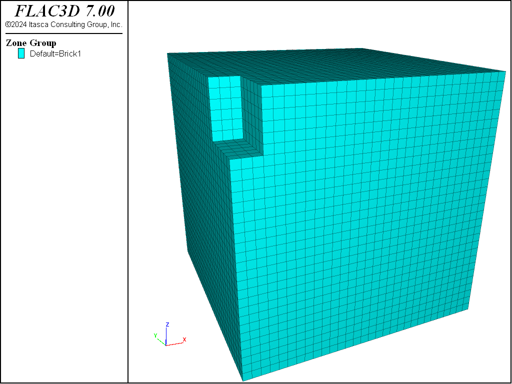
Figure 1: Cartoon model of a trench excavation.
The full data file for the first demonstration is below. Note that zone relax excavate was deliberately not used for the purposes of illustration.
model new
model large-strain off
; Create zones
zone create brick size 30 30 30
zone face skin
zone group 'Trench' range position (0,0,24) (3,6,30)
; Constitutive model and properties
zone cmodel assign mohr-coulomb
zone property bulk 3e6 shear 2e6 density 1000
zone property cohesion 1e5 friction 25 tension 1e3
zone cmodel assign elastic range group 'Wall'
zone property bulk 3e6 shear 2e6 density 1000
; Boundary conditions
zone face apply velocity-normal 0 range group 'East' or 'West'
zone face apply velocity-normal 0 range group 'North' or 'South'
zone face apply velocity-normal 0 range group 'Bottom'
; Initial conditions
model gravity 10
zone initialize-stresses
model solve
; Histories
model history mechanical ratio-average
zone history displacement-x position (3,0,30)
zone history displacement-z position (4,0,30)
; Excavate
zone delete range group 'Trench'
; Solve
model solve
model save 'simple'
There are several things that should always be done to check to see if your model has actually reached sufficient equilibrium. First, take histories of displacements and/or velocities in regions of primary interest. If these displacements are still changing relatively rapidly when cycling completes, the model is not done adjusting. Second, make plots (contours and isosurfaces) of Local Force Ratio or Convergence. An isosurface plot of Convergence is particularly useful to tell you where the model is taking the longest to converge, and where you should look closer in a contour plot (perhaps using cut-planes to see into the interior of the model).
Figure 2 shows the histories of averaged force ratio and displacements in the top of the trench. Note that the average force ratio is plotted on a log scale. For a well-behaved model, this sort of linear logarithmic (or exponential) convergence is expected. Failure or other non-linear behavior will show disturbances in convergence, and progressive uncontained failure will make the curve level out. The displacement history, again, shows a typical slightly underdamped response. It is clear that the top of the trench wall has stopped moving significantly and the model has effectively reached equilibrium.
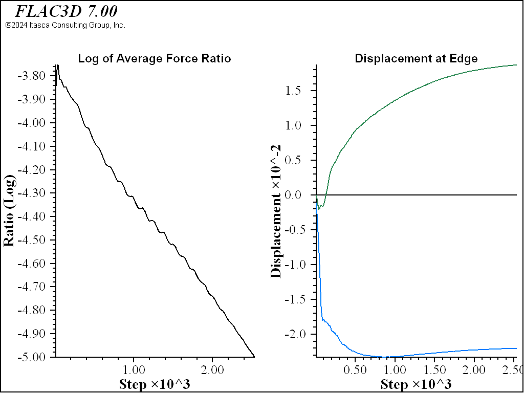
Figure 2: Histories of average unbalanced ratio and displacement for the simple trench.
Figure 3 shows the result of examining contours of convergence. While the bulk of the model has a convergence well below 1, a few gridpoints near the surface are still much higher. This is fairly typical of this sort of problem; the surface gridpoints have the same inertial mass resisting motion and smaller driving forces due to stress. The gridpoints at the bottom tend to (and need to) converge first, and small adjustments propagate against gravity, so the surface gridpoints converge last. If a stricter convergence criteria of convergence 1 was used, the model would take half again as many steps to reach equilibrium. How important this is depends on the significance of relatively small adjustments in the surface gridpoints. If exact surface settlement values were critical, this might be a necessary change.
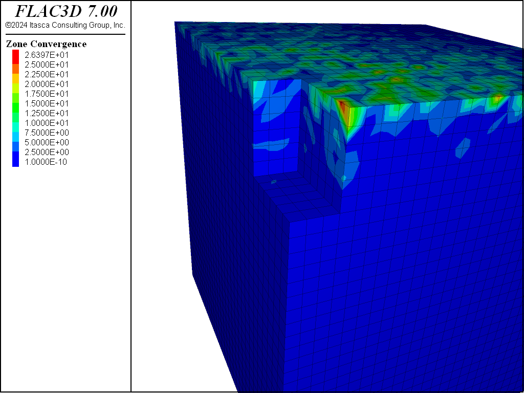
Figure 3: Contours of gridpoint convergence.
Effects of Large Stiffness Differences
To illustrate some of the possible difficulties, we introduce a large localized stiffness difference by adding a steel liner to the trench after excavation. The complete data file for this modification is shown below.
-model new
model large-strain off
; Create zones
zone create brick size 30 30 30
zone face skin
zone group 'Trench' range position (0,0,24) (3,6,30)
zone face group 'Wall' internal ...
          range group 'Brick1' group 'Trench' position-z 24.1 30
; Constitutive model and properties
zone cmodel assign mohr-coulomb
zone property bulk 3e6 shear 2e6 density 1000
zone property cohesion 1e5 friction 25 tension 1e3
; Boundary conditions
zone face apply velocity-normal 0 range group 'East' or 'West'
zone face apply velocity-normal 0 range group 'North' or 'South'
zone face apply velocity-normal 0 range group 'Bottom'
; Initial conditions
model gravity 10
zone initialize-stresses
model solve
; Histories
model history mechanical ratio-average
zone history displacement-x position (3,0,30)
zone history displacement-z position (4,0,30)
; Excavate
zone delete range group 'Trench'
; Install liner
struct shell create by-zone-face range group 'Wall'
struct shell property isotropic 10e9 0.1 thick 1
model solve
model save 'stiff'
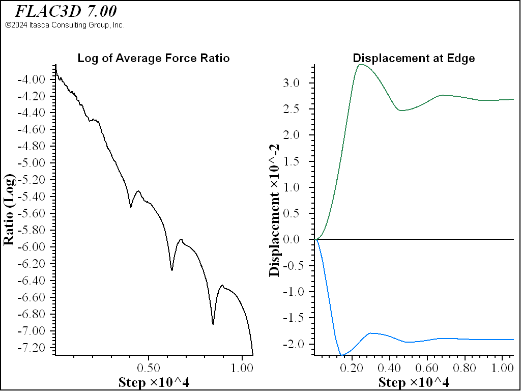
The histories for the modified model are shown in Figure 4. While the average force ratio shows similar characteristics, the histories indicate that the model has not settled down into equilibrium. The issue is that the very stiff structural wall results in high inertial masses (see Mechanical Timestep Determination for Numerical Stability), while the forces driving settlement remain the same. This means the gridpoints connected to the shell elements move relatively slowly, and their convervence values lag behind the rest of the model. Eventually, this localized disturbance can be drowned out by the bulk of the model, and on average, the model will appear converged.
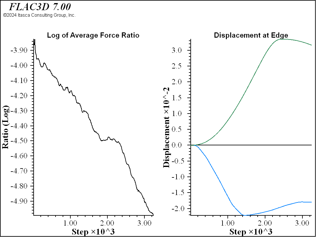
Figure 4: Histories of average unbalanced ratio and displacement for a trench with a stiff reinforcing wall.
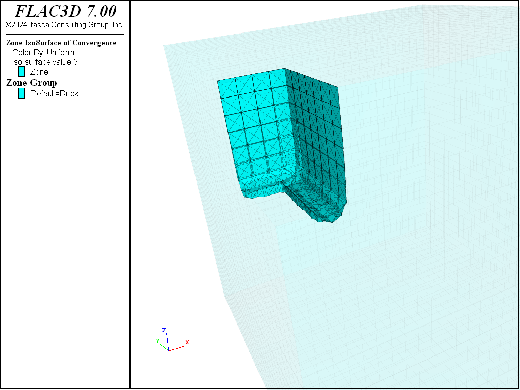
Figure 5: Isosurface of Convergence 5.
An isosurface plot of Convergence shown in Figure 5 reveals that the area around the wall is having trouble coming to equilibrium. If the convergence criteria used was changed to
plot 'Isosurface' export bitmap filename 'Isosurface.png' -skip-test
then the model would take much longer, but would also reach a state where there was some confidence that equilibrium had been achieved, as seen in Figure 6.
| Was this helpful? ... | FLAC3D © 2019, Itasca | Updated: Feb 25, 2024 |