Initial Conditions
In all civil or mining engineering projects, there is an in-situ state of stress in the ground, before any excavation or construction is started. In FLAC3D, an attempt is made to reproduce this in-situ state by setting initial conditions. Ideally, information about the initial state comes from field measurements. But, when these are not available, the model can be run for a range of possible conditions. Although the range is potentially infinite, there are a number of constraining factors (e.g., the system must be in equilibrium, and the chosen yield criteria must not be violated anywhere).
In a uniform layer of soil or rock with a free surface, the vertical stresses are usually equal to \(gρz\), where \(g\) is the gravitational acceleration, \(ρ\) is the mass density of the material, and \(z\) is the depth below the surface. However, the in-situ horizontal stresses are more difficult to estimate. There is a common—but erroneous—belief that there is some “natural” ratio between horizontal and vertical stress, given by \(ν/(1-ν)\), where \(ν\) is the Poisson’s ratio. This formula is derived from the assumption that gravity is suddenly applied to a mass of elastic material in which lateral movement is prevented. This condition hardly ever applies in practice, due to repeated tectonic movements, material failure, overburden removal and locked-in stresses due to faulting and localization (see Localization, Physical Instability, and Path-Dependence). Of course, if we had enough knowledge of the history of a particular volume of material, we might simulate the whole process numerically to arrive at the initial conditions for our planned engineering works, but this approach is not often feasible. Typically, we compromise: a set of stresses is installed in the grid, and then FLAC3D is run until an equilibrium state is obtained. It is important to realize that there are an infinite number of equilibrium states for any given system.
In the following topics, we examine progressively more complicated situations and the ways in which the initial conditions may be specified. The user is encouraged to experiment with the various data files presented.
Uniform Stresses — No Gravity
For an excavation deep underground, the gravitational variation of stress from top to bottom of
the excavation may be neglected because the variation is small in comparison to the magnitude of
stress acting on the volume of rock to be modeled. The model gravity command may be
omitted, causing the gravitational acceleration to default to zero. Initial uniform stresses
can be installed with the zone initialize command. For example, the commands
zone initialize stress-xx -5e6
zone initialize stress-yy -1e7
zone initialize stress-zz -5e6
will set the stress components \(\sigma_{xx}\), \(\sigma_{yy}\), and \(\sigma_{zz}\) to compressive stresses of -5 × 10⁶, -107, and -5 × 10⁶, respectively, throughout the grid. Range parameters may be added if the stresses are to be restricted to a sub-grid.
The stress keyword can be used to initialize the entire stress tensor at once. This can only be done for a uniform stress field. The following is almost the equivalent command:
zone initialize stress xx -5e6 yy -1e7 zz -5e6
The difference is that the stress keyword initializes all six components of stress for each zone in the range. Components that were not explicitly assigned a value are assumed to be zero.
The zone initialize command sets all stresses to the given values, but there is no
guarantee that the stresses will be in equilibrium. There are at least two possible problems.
First, the stresses may violate the yield criterion of a nonlinear model that has been assigned
to the grid. In this case, plastic flow will occur immediately upon cycling and the stresses
will readjust. This possibility should be checked by doing one trial step and examining the
response (e.g., create zone plot item, set “ColorBy” to “Label”, and set “Label” to “State”).
Second, the prescribed stresses at the grid boundary may not equal the given initial stresses.
In this case, the boundary gridpoints will start to move as soon as cycling begins. Again,
output should be checked (e.g., plot a zone-vectors plot item, set “Value” to “Velocity”) for
this possibility. The example below shows a set of commands that produce initial stresses that
are in equilibrium with prescribed boundary stresses.
Initial and boundary stresses in equilibrium
model new
zone create brick size 6 6 6
zone face skin
zone cmodel assign elastic
zone initialize stress xx=-5e6 yy=-1e7 zz=-2e7
zone face apply stress-xx=-5e6 range group 'East' or 'West'
zone face apply stress-yy=-1e7 range group 'North' or 'South'
zone face apply stress-zz=-2e7 range group 'Top' or 'Bottom'
Of course, if the boundary is velocity rather than stress-controlled, the initial stresses will
be in equilibrium automatically; the zone face apply command is not necessary. See
Boundary Conditions for more details on boundary conditions and the zone apply and zone face apply commands in particular.
Stresses with Gradients — Uniform Material
Near the ground surface, the variation in stress with depth cannot be ignored. The
model gravity command is used to inform FLAC3D that gravitational acceleration operates
on the grid. It is important to understand that the model gravity command does not
directly cause stresses to appear in the grid; it simply causes body forces to act on all
gridpoints. These body forces correspond to the weight of material surrounding each gridpoint.
If no initial stresses are present, the forces will cause the material to move (during stepping)
in the direction of the forces until equal and opposite forces are generated by zone stresses.
Given the appropriate boundary conditions (e.g., fixed bottom, roller side boundaries), the
model will, in fact, generate its own gravitational stresses that are compatible with the
applied gravity. However, this process is inefficient, since many hundreds of steps may be
necessary for equilibrium. It is better to initialize the internal stresses such that they
satisfy both equilibrium and the gravitational gradient.
The zone initialize-stresses command will automatically initialize a stress field due to
gravity. The model gravity command must have been given first, and density must
have been assigned to all zones. zone initialize-stresses calculates stresses
regardless of any irregularity in the geometry. It works by finding all changes in values that
affect gravitational loading and tracking which ones are crossed as you move from a given zone
against the direction of gravity.
Initial stress state with gravitational gradient
model gravity 10
zone initialize-stresses ratio 0.5
zone face apply stress-normal [-1000*10*10*0.5] ...
                gradient (0,0,[1000*10*0.5]) ...
The ratio keyword specifies a horizontal stress ratio \(K_0\) that is used to determine the \(\sigma_{xx}\) and \(\sigma_{yy}\) stresses that in this case are equal. Note that if stress boundary conditions are used, they need to be compatible with the stresses calculated by zone initialize-stresses. In this case, in-line FISH can be used to make the load and gradient calculations clear and simple. The maximum compressive vertical stress is the height * density * gravity * ratio, and the gradient is density * gravity * ratio. Note that the simple model in question is a 10 m × 10 m × 10 m box of homogeneous material, and the top surface is free.
The following zone initialize command is, for this particular instance, functionally the same as zone initialize-stresses
model solve
zone initialize stress-xx [-1000*10*10*0.5] gradient (0,0,[1000*10*0.5])
zone initialize stress-yy [-1000*10*10*0.5] gradient (0,0,[1000*10*0.5])
In this example, horizontal stresses and gradients are equal to half the vertical stresses and gradients, but they may be set at any value that does not violate the yield criterion (Mohr-Coulomb, in this case). After preparing a data file such as the one shown here, one calculation step should be executed and the velocity field plotted; any failure to match internal stresses with boundary stresses will show up as a systematic movement at one or more boundaries. Small, chaotic velocities may be ignored (see Interpretation: Gridpoint Velocities). The unbalanced force after one step will be very small, but may not be exactly zero. This is a function of round-off error.
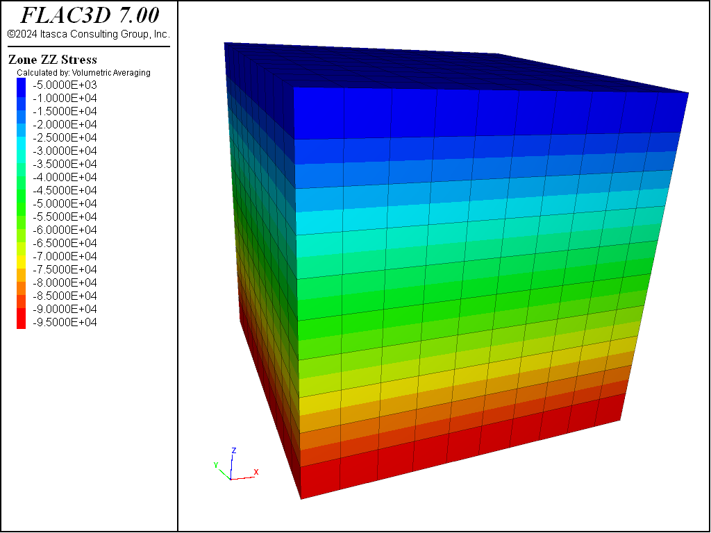
Figure 1: Uniform gradient equilibrium vertical stresses.
Note that the gradient specified with the gradient keyword associates stresses with zone centroids (i.e., the global location of the centroid determines the stress value from the gradient). Thus, although the applied \(\sigma_{xx}\)-stress varies from -5.0 × 10⁶ to -4.5 × 10⁶ in the example above, the actual zone stresses in this example vary from -4.975 × 10⁶ to -4.525 × 10⁶. The stress-contours may be plotted with or without interpolation of the zone stress from the centroid to the boundary; the stress at the boundary is not exactly the stress in the boundary zone. To see the differences, plot a zone plot item, set “ColorBy” to “Contour”, “Value” to “Stress”, and “Quantity” to “zz”. Then change the selection on the “Method” attribute (options are “Constant”, “Volumetric Averaging”, “Inv. Distance Weighting”, and “Polynomial Extrapolation”) and note the result. Actual stresses in the zone are shown when the “Method” is set to “Constant”.
Stresses with Gradients — Nonuniform Material
zone initialize-stresses should generally be used to find initial stresses in more difficult models when materials of different densities are present. Consider a layered system with a free surface, enclosed in a box with roller side boundaries and fixed base. Suppose that the material has the following density distribution:
1600 kg/m3 from 0 to 10 m depth
2000 kg/m3 from 10 to 15 m
2200 kg/m3 from 15 to 25 m
An equilibrium state is produced by the following data file.
Initial stress gradient in a nonuniform material
model new
model large-strain off
; Create Zones
zone create brick size 10 10 10 ...
                  point 0 (0, 0,0) point 1 (20,0, 0) ...
                  point 2 (0,20,0) point 3 ( 0,0,25)
zone face skin
; Constitutive model and properties
zone cmodel assign elastic
zone property bulk 5e9 shear 3e9
zone initialize density 1600 range position-z  0 10
zone initialize density 2000 range position-z 10 15
zone initialize density 2200 range position-z 15 25
; Boundary Conditions
zone face apply velocity-normal 0 range group 'East' or 'West'
zone face apply velocity-normal 0 range group 'North' or 'South'
zone face apply velocity-normal 0 range group 'Bottom'
zone face apply stress-normal -1e6 range group 'Top'
; Initial Conditions
model gravity 10
zone initialize-stresses ratio 0.25 0.5 overburden -1e6
model solve
Without the use of zone initialize-stresses, the stress at each material interface must be calculated manually from the known overburden above it. This is somewhat tractable for a simple layered material, using the gradient formula to calculate the value following stress-zz on the zone initialize command. The gradient values are simply the variations across each layer due to the gravitational gradient. In this example, an overburden of -1e6 was added to the surface, and a different horizontal stress ratio was used in the \(\sigma_{xx}\) and \(\sigma_{yy}\) direction.
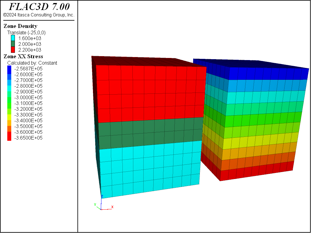
Figure 2: Nonuniform densities and resulting equilibrium vertical stresses.
In a more complicated situation, if zone initialize-stresses was not suitable for some reason, it would be necessary to use a FISH function to compute initial approximate stress values from a known material property distribution.
Stress Initialization in a Nonuniform Material
The existence of internal nonuniformities in a FLAC3D grid should not change the way stresses are initialized. However, some minor adjustment may be necessary, because forces do not balance exactly if the grid is irregular. For example, a grid may be distorted internally into the shape of a cylinder, with a view to “excavating” a tunnel at some later stage in the run. There will be a very slight initial imbalance in forces, but this may be relaxed with a few steps, as illustrated in this example.
Initial stress state for a nonuniform grid
model new
model large-strain off
; Create grid
zone create radial-cylinder size 3 8 4 5 fill ...
            point 1 (10,0,0) point 2 (0,10,0) point 3 (0,0,10)
zone face skin
; Constitutive model and properties
zone cmodel elastic
zone property shear 3e8 bulk 5e8 density 2500
; Boundary conditions
zone face apply velocity-normal 0 range group 'East' or 'West'
zone face apply velocity-normal 0 range group 'North' or 'South'
zone face apply velocity-normal 0 range group 'Bottom'
; Initial conditions
model gravity 10
zone initialize-stresses
model solve
At one calculation step, the unbalanced force ratio is approximately 3.5e-3. It takes approximately 200 additional steps for this to be reduced to 1e-5. The final zone stresses and displacements resulting from this adjustment are shown below.
More complications arise when a free surface has an irregular geometry. The next example produces the “mountain range” shown in the figure that follows, using the zone generate from-topography command.
Initial stress state for an irregular surface
model new
model large-strain off
; Create Zones
zone create brick size 30 30 10 point 0 (0,0,0) point 1 (580,0,0) ...
                                point 2 (0,680,0) point 3 (0,0,100)
geometry import 'test.stl'
zone generate from-topography direction (0,0,1) geometry-set 'test' segments 20
zone face skin
; Constitutive model and properties
zone cmodel assign elastic
zone property bulk 3e8 shear 2e8 density 1000
; Boundary conditions
zone face apply velocity-normal 0 range group 'East' or 'West'
zone face apply velocity-normal 0 range group 'North' or 'South'
zone face apply velocity-normal 0 range group 'Bottom'
; Initial conditions
model gravity 10
zone initialize-stresses ratio 0.5
model solve elastic
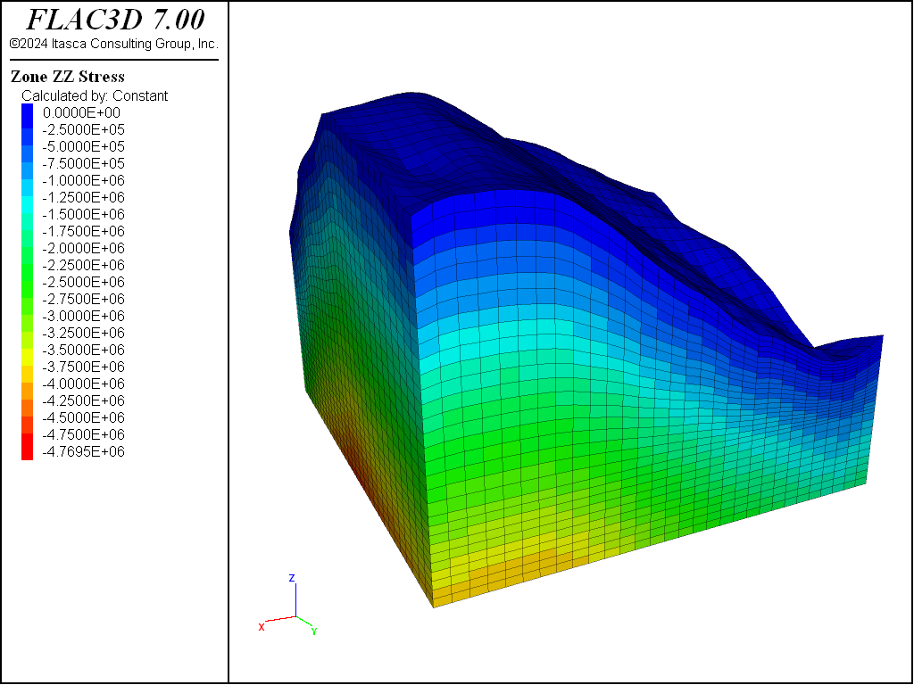
Figure 4: Initialized stresses in an irregular topological grid in FLAC3D.
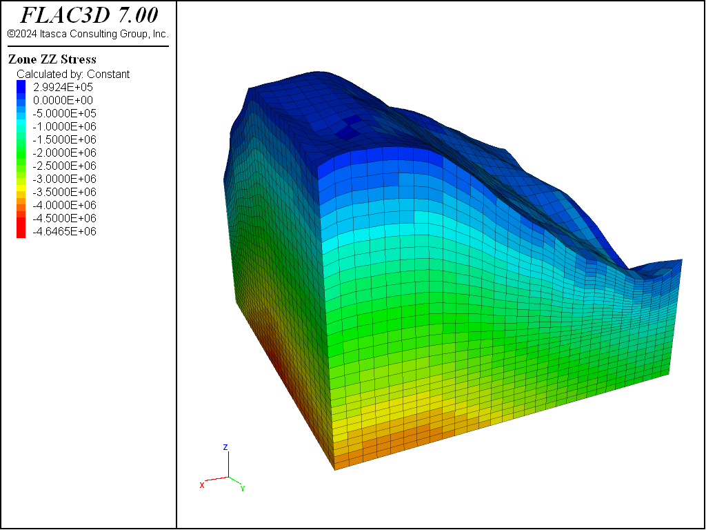
Figure 5: Stresses after cycling to equilibrium.
The zone initialize-stresses command calculates an approximate vertical stress
distribution for the model, which is very close to actual equilibrium. If the horizontal stress
ratio were set to 0, it would only take approximately 200 steps to reach full
equilibrium after initialization. With a finite stress ratio in a surface topography like this,
however, problems occur. A horizontal stress ratio that is perfectly correct near the base is
generally too high when near the surface of a slope. This can take some time to come to
equilibrium and can also cause unrealistic displacement or even damage on surface slopes.
There is no simple way to calculate initial stresses that are nearer equilibrium for this case. There are a number of different possible methods one could use to help, however:
- Use multiple
zone initialize-stressescommands at different elevations and regions, with different ratio values.- Solve the model elastically.
- Reset displacement after reaching initial equilibrium (this is generally good practice in any case).
- Allow plastic flow to occur, thus removing stress concentrations, and then re-assign constitutive models to reset state variables.
There are probably many other possible schemes, particularly for a nonlinear, path-dependent material. No initial state is the “correct one”: the choice may depend on the type of geological process that is believed to have occurred in the field.
Compaction within a Nonuniform Grid
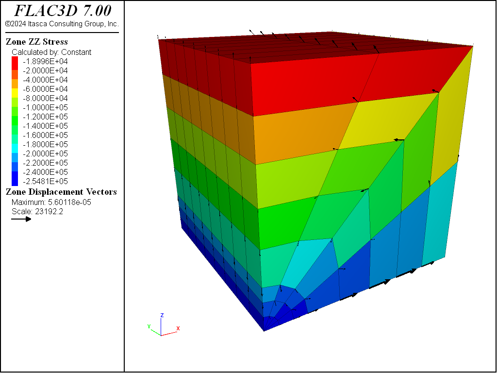
Puzzling results are sometimes observed when a model is allowed to come to equilibrium under gravity, using a nonuniform grid. When a Mohr-Coulomb or other nonlinear constitutive model is used, the final stress state and displacement pattern are not uniform, even though the boundaries are straight and the free surface is flat. The data file in the following example illustrates the effect (see the figure following for the generated plot showing displacement vectors and vertical stress contours).
Nonuniform stress initialized in nonuniform grid
model new
model large-strain off
; Create zones
zone create brick size 8 8 10 ratio 1.2 1 1
zone face skin
; Constitutive model and properties
zone cmodel assign mohr-coulomb
zone property bulk 2e8 shear 1e8 friction 30 density 2000
; Boundary Conditions
zone face apply velocity-normal 0 range group 'East' or 'West'
zone face apply velocity-normal 0 range group 'North' or 'South'
zone face apply velocity-normal 0 range group 'Bottom'
model gravity 10
model save 'initial'

; -- the following lines will produce nonuniform patterns:
model solve
model save 'nonuniform'

; -- the following lines set stresses directly:
model restore 'initial'
zone initialize-stresses ratio 0.75
model solve
model save 'direct'

; -- the following lines initialize elastically:
model restore 'initial'
model solve elastic
model save 'uniform'

Figure 6: Nonuniform stresses and displacements.
Because we have roller boundaries on the vertical sides, we might expect the material to move down equally on these sides. However, the grid is finer near the origin. FLAC3D tries to keep the local timestep equal for all zones, so it increases the inertial mass for the gridpoints near the \(x\) = 0 boundary to compensate for the smaller zone sizes. These gridpoints then accelerate more slowly than those near the \(x\) = 8 boundary. This will have no effect on the final state of a linear material, but it causes nonuniformity in a material that is path-dependent. For a Mohr-Coulomb material without cohesion, the situation is similar to dropping sand from some height into a container and expecting the final state to be uniform. In reality, a large amount of plastic flow would occur because the confining stress does not build up immediately. Even with a uniform grid, this approach is not a good one because the horizontal stresses depend on the dynamics of the process.
The best solution is to use the zone initialize-stresses command to set initial stresses
to conform to the desired \(K\)0 value (ratio of horizontal to vertical stresses).
For example, the model solve command in the previous data file would stop immediately if
it was preceded by the line
model restore 'initial'
A stable state is achieved with \(K\)0 = 0.75; no stepping is necessary.
If for some reason it is desirable to use FLAC3D to compute the final state, then the
model solve elastic option could be used. This solves the model to equilibrium without
allowing any plastic failure in the constitutive model, then re-activates failure and makes
certain the model remains in equilibrium.
model restore 'initial'
The next figure shows the displacement vectors and vertical stress contours for this case. The material is prevented from yielding during the compaction process, but the original properties are restored when equilibrium is achieved.
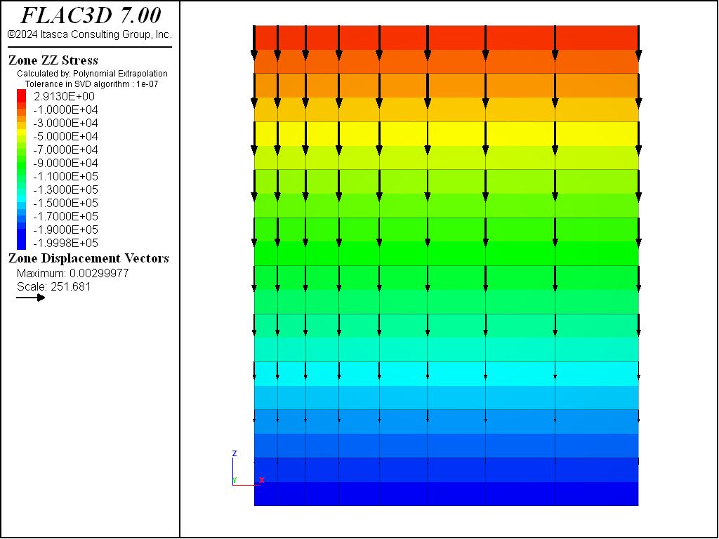
Figure 7: Uniform stresses and displacements.
Initial Stresses following a Model Change
There may be situations in which one constitutive model is used in the process of reaching a desired stress distribution, but another constitutive model is used for the subsequent simulation. If one cmodel is replaced by another non-null cmodel, the stresses in the affected zones are preserved, as in this example:
Initial stresses following a model change
model new
model large-strain off
; Create zones
zone create brick size 5 5 5
zone face skin
zone group 'Switch' range position (0,0,0) (2,5,2)
; Constitutive models and properties
zone cmodel assign elastic
zone property shear 2e8 bulk 3e8 density 2000
; Boundary conditions
zone face apply velocity-normal 0 range group 'Bottom'
model gravity 10
zone initialize-stresses
model solve
zone cmodel assign mohr-coulomb range group 'Switch'
zone property shear 2e8 bulk 3e8 friction 35 range group 'Switch'
model step 1000
At this point in the run, the stresses generated by the initial elastic model still exist and act as initial stresses for the region containing the new Mohr-Coulomb model.
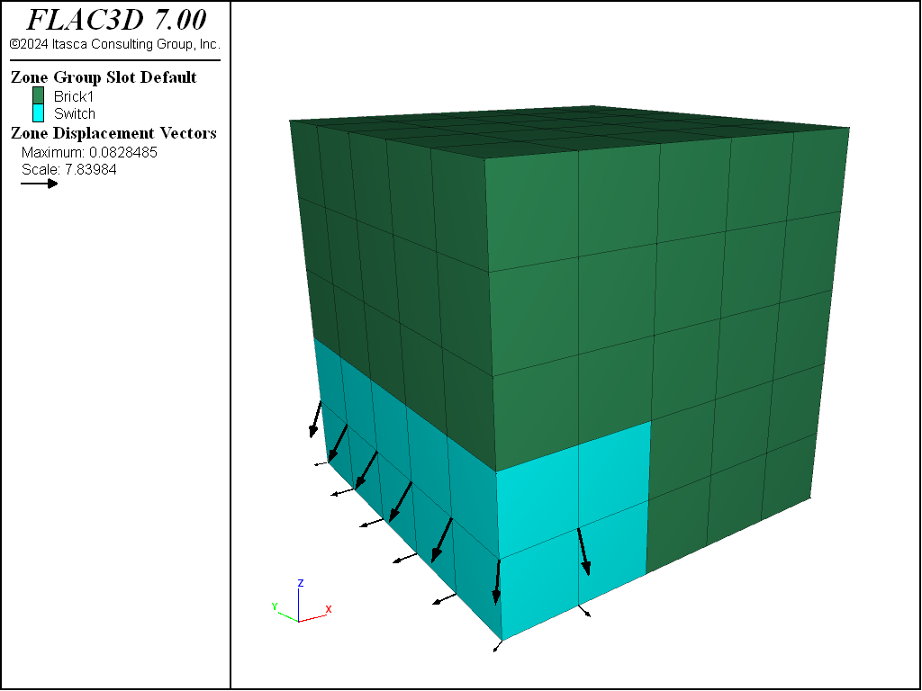
Figure 8: Area of constitutive model change and displacements resulting from failure.
Two points should be remembered:
First, if a null model is installed in any zones (even if it is subsequently replaced by another model), all stresses are removed from the affected zones.
Second, if one model is replaced by another and the stresses should physically be zero in the new model, then a
zone initializecommand must be used to reset the stresses to zero. This situation would occur if rock is mined out and replaced by backfill; the backfill would have its own stress state, unrelated to the rock it is replacing.
Stress and Pore-Pressure Initialization with a Phreatic Surface
Pore pressures are initialized in the same way as stresses. However, the gridpoint pore
pressures, rather than the zone pore pressures, are initialized regardless of whether
model configure fluid is specified. Zone pore pressures are derived from gridpoint pore
pressures by averaging. Zone pore pressures are then used to calculate effective stresses needed
by the constitutive models.
Manual initialization of a partially saturated grid can be confusing; it is very important to remember two things:
- If the grid has not been configured for groundwater calculations, then densities specified below the phreatic surface (pore-pressure = 0) must be wet densities and those above the phreatic surface must be dry densities. It is up to the user to supply proper values for densities in those regions.
- If the grid has been configured for groundwater calculations (
model configure fluid), then dry densities are specified everywhere and the contribution from the fluid is calculated automatically from the porosity, saturation, and fluid density.
If the proper material properties for each case have been specified (dry
density/porosity/saturation/fluid density for model configure fluid, wet/dry density
distribution otherwise), then the zone initialize-stresses command will automatically
calculate the correct vertical stress including the weight of fluid.
Note that the \(\kappa_0\) calculated using the ratio keyword is done using effective stresses. Use the total keyword to calculate horizontal stress ratios in terms of total stresses.
Below are short examples illustrating each case.
Stress and pore pressure initialization with a phreatic surface — grid not configured for groundwater
model new
model large-strain off
; Create zones
zone create brick size 8 5 10
zone face skin
; Mech constitutive model and properties
zone cmodel assign elastic
zone property bulk 1e9 shear 5e8 density 2000
zone property density 2500 range position-z 0 5 ; Wet Density
zone property density 2250 range position-z 5 6 ; Partially saturated density
; Boundary Conditions
zone face apply velocity-normal 0 range group 'East' or 'West'
zone face apply velocity-normal 0 range group 'North' or 'South'
zone face apply velocity-normal 0 range group 'Bottom'
; Initial conditions
model gravity 10
zone water density 1e3
zone water plane origin (0,0,5) normal (0,0,1)
zone initialize-stress ratio 0.5
model solve ; immediately at equilibrium
In this example, the density was adjusted on and below the phreatic surface to partially saturated and wet values.
Stress and pore pressure initialization with a phreatic surface — grid configured for groundwater
model new
model large-strain off
model config fluid
; Create zones
zone create brick  size 8 5 10
zone face skin
; Mech constitutive model and properties
zone cmodel assign elastic
zone property bulk 1e9 shear 5e8 density 2000
; Fluid constitutive model and properties
zone fluid cmodel assign isotropic
zone fluid property porosity 0.5 permeability 1e-10
zone gridpoint initialize fluid-modulus 2e9
zone initialize fluid-density 1e3
; Boundary Conditions
zone face apply velocity-normal 0 range group 'East' or 'West'
zone face apply velocity-normal 0 range group 'North' or 'South'
zone face apply velocity-normal 0 range group 'Bottom'
; Initial conditions
model gravity 10
zone water density 1e3
zone water plane origin (0,0,5) normal (0,0,1)
zone gridpoint initialize saturation 0 range position-z 5.1 10
zone initialize-stress ratio 0.5
model solve ; immediately at equilibrium
There are a few things to note in this example. First, the saturation needs to be explicitly
initialized to zero above the phreatic surface. Second, as noted above, the dry density was
given everywhere. Third, the zone water command was used to initialize pore pressures,
which requires that a fluid density be given separately from the
zone initialize fluid-density command.
Initialization of Velocities
Until now, we have concentrated on initialization of stresses. Normally, the velocities inside the grid are not set explicitly; they default to zero initially. If, however, a velocity loading condition is specified at the boundary of a body, it is sometimes beneficial to initialize the velocities throughout the body to minimize the shock to the system. For example, in a simulated triaxial test with rigid platens, the velocities can be initialized to achieve an initial linear gradient throughout the sample, as shown in the following example.
Velocity gradient in a triaxial test
model new
model large-strain off
; Create zones
zone create cylinder point 0 (0,0,0) point 1 (1,0,0) ...
                     point 2 (0,2,0) point 3 (0,0,1) ...
                     size 4 5 4
zone reflect normal (1,0,0)
zone reflect normal (0,0,1)
zone face skin
; Constitutive model and properties
zone cmodel assign mohr-coulomb
zone property bulk 1.19e10 shear 1.1e10
zone property cohesion 2.72e5 friction 44 tension 2e5
; Boundary conditions
zone face apply velocity-normal -1e-4 range group 'North'
zone face apply velocity-normal 0 range group 'South'
zone face apply stress-normal -1e5 range group 'East'
; Velocities initialized to smooth response.
zone gridpoint initialize velocity-y 0 gradient (0,-1e-4,0)
If the linear gradient is not applied, the internal gridpoints will receive an initial shock because they must accelerate to produce a negative velocity through the sample. The subsequent motion of the internal gridpoints is not controlled, because only the ends are fixed.
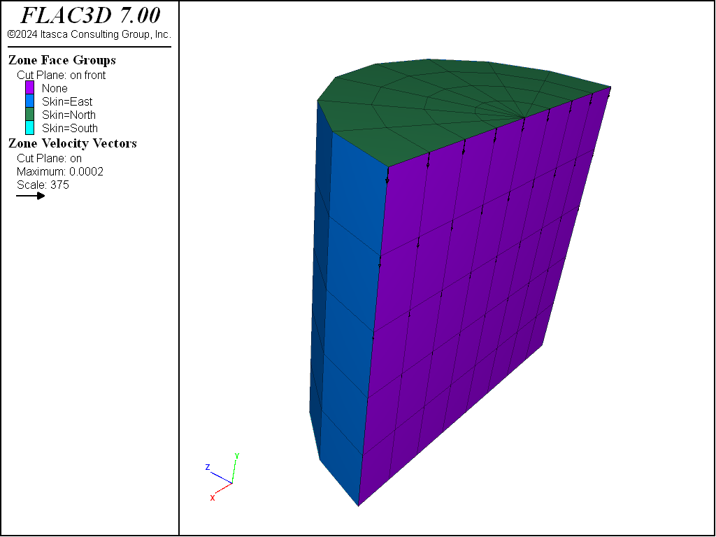
Figure 9: Velocities initialize in simple triaxial test sample.
| Was this helpful? ... | FLAC3D © 2019, Itasca | Updated: Feb 25, 2024 |