Verification of Concepts, and Modeling Techniques for Specific Applications
Solid Weight, Buoyancy and Seepage Forces
When fluid flows through a porous medium there are, following Terzaghi (1943) and Taylor (1948), three forces acting per unit volume on the solid matrix: the solid weight, the buoyancy, and the drag or seepage force (also see Bear 1972). These forces are automatically taken into account in the FLAC3D formulation. This may be shown as follows.
In FLAC3D, equilibrium is expressed using total stress:
where \(\rho_s\) is the undrained (saturated bulk) density, and \(g_i\) is the gravitational vector. (Note that Einstein notation convention for summation over repeated indices applies to the equations in this section.) Undrained density may be expressed in terms of drained density, \(\rho_d\), and fluid density, \(\rho_w\), using the expression
where \(n\) is porosity, and \(s\) is saturation. The definition of effective stress is
Substitution of Equation (2) and Equation (3) in Equation (1) gives, after some manipulations,
where we have introduced fluid unit weight, \(\gamma_w\), and piezometric head, \(\phi\), as
and \(g\) is the gravitational magnitude.
In Equation (4), the term \(\rho_d g_i\) can be associated with solid weight, \((1-n) {\partial p \over \partial x_i}\) with buoyancy, and \(n \gamma_w {\partial \phi \over \partial x_i}\) with seepage force (drag).
A Simple Example Illustrating Solid Weight, Buoyancy and Seepage Forces
A simple example is given below to illustrate the contribution of these individual terms in the context of FLAC3D methodology. We consider a layer of soil of large lateral extent and thickness, \(H\) = 10 m, resting on a rigid base. The layer is elastic, the drained bulk modulus, \(K\), is 100 MPa, and the shear modulus, \(G\), is 30 MPa. The density of the dry soil, \(\rho_d\), is 500 kg/m3. The porosity, \(n\), is uniform with a value of 0.5. The mobility coefficient, \(k\), is 10-8 m2/(Pa-sec). The fluid bulk modulus, \(K_w\), is 2 GPa, and gravity is set to 10 m/sec2.
Initially, the water table is at the bottom of the layer, and the layer is in equilibrium under gravity. We study the heave of the layer when the water level is raised, and also the heave or settlement under a vertical head gradient.
The problem is one dimensional; the FLAC3D model is a mesh composed of a single column of 10 zones in the \(z\)-direction. The axes origin is at the bottom of the model. The mechanical boundary conditions correspond to roller boundaries at the base and sides of the model. The fluid-flow boundary conditions are described for the individual cases below.
This example is run using the groundwater configuration (model configure fluid).
The coupled groundwater-mechanical calculations are performed using the basic fluid-flow scheme.
The calculation times are quite short for this small model;
for larger models, uncoupled modeling can be applied to speed the calculation.
For reference, in a comparison of FLAC3D results to the analytical solutions, the one-dimensional incremental stress-strain relation for this problem condition is
where \(\alpha\) is the Biot coefficient (set equal to 1 for this simulation), \(K\) is the drained bulk modulus, \(G\) is the shear modulus, and \(\epsilon_{zz}\) is the vertical strain.
Solid Weight — We first consider equilibrium of the dry layer.
The dry density of the material is assigned, and the saturation is initialized to zero
(the default value for saturation is 1 in model configure fluid mode).
The flow calculation is turned off, and the mechanical calculation is on.
The value of fluid bulk modulus is set to zero to prevent any generation of pore pressure under volumetric straining for this stage.
The model is cycled to equilibrium.
By integration of Equation (1) applied to the dry medium, we obtain
Vertical stress at the end of the FLAC3D simulation is plotted versus elevation in Figure 1. The values match those obtained for equilibrium under gravity of the dry medium (Equation (8)), as expected.
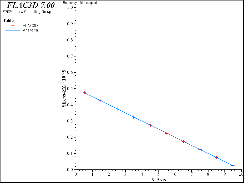
Figure 1: Vertical stress versus elevation — dry layer.
The vertical displacement at the top of the model is found from the equation.
The calculated value from FLAC3D matches the analytical value at this stage (-1.786 × 10⁻³ m).
Note that the equilibrium ratio limit (model solve mechanical ratio) is reduced to 10-6 to provide this level of accuracy for this example.
Buoyancy — We continue this example by raising the water table to the top of the model. We reset the displacements to zero, and assign the fluid properties listed above. The pore pressure is fixed at zero at the top of the model, and the saturation is initialized to 1 throughout the grid. (Note that a fluid-flow calculation to steady state is faster if the state starts from an initial saturation 1 instead of a zero saturation.) Fluid-flow and mechanical modes are both on for this calculation stage, and a coupled calculation is performed to reach steady state. The code uses the saturated density for this calculation, as determined (internally) from Equation (2). By integration of Equation (1) for the saturated medium, we obtain
The comparison of total vertical stress profile from FLAC3D to that from Equation (10) is shown in Figure 2:
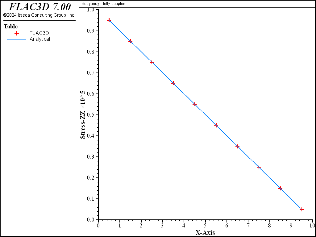
Figure 2: Vertical stress versus elevation — saturated layer.
At steady state, the pore pressure is hydrostatic:
Contours of pore pressure at steady state are shown in Figure 3.
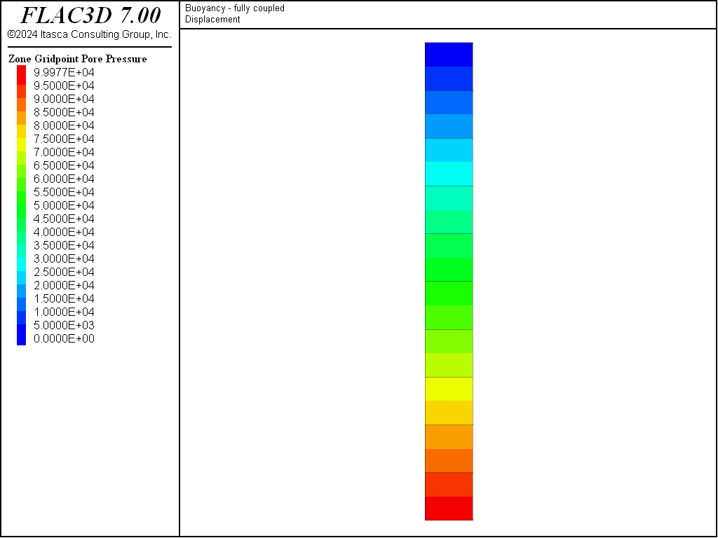
Figure 3: Pore pressure contours at steady state — saturated layer.
The vertical displacement induced by raising the water table is now upwards. The amount of heave is calculated starting from Equation (7). We write this equation in the form
For this example, \(p^{(1)}\) = 0. After substitution of Equation (8), Equation (10) and Equation (11) into Equation (12), we obtain, after some manipulation,
The term \((\rho_s - \rho_w)\) is the buoyant density. Substitution of Equation (2) for undrained density in Equation (13) produces
Finally, after integration between 0 and H, we obtain
and, for \(z = H\), this gives
The final numerical displacement at the top of the model compares well with the analytical value (+1.786 × 10⁻³ m). The displacements, induced upward, are plotted in Figure 4:
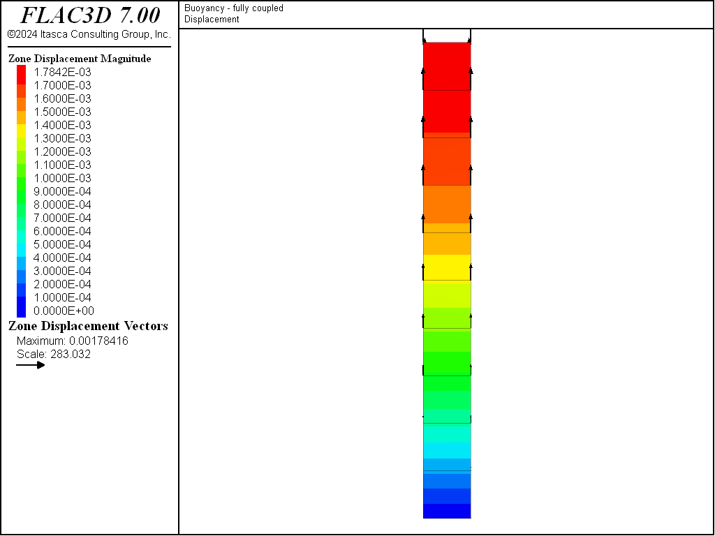
Figure 4: Heave of the layer at steady state — saturated layer.
Additional Rise in Water Table — We continue from this stage, and model the effect of an additional rise in the water level on the layer. This time, the water table is raised to 20 m above the top of the model. The corresponding hydrostatic pressure is \(p = \rho_w g h\), where \(h\) is 20 m and \(p\) = 0.2 MPa.
We reset displacements to zero and apply a pressure of 0.2 MPa at the top of the model.
A fluid pore pressure is applied (with zone gridpoint fix pore-pressure 2e5),
as is a mechanical pressure (with zone face apply stress-normal), along the top boundary.
We now perform the coupled calculation again for an additional 500 seconds of fluid-flow time.
No further movement of the model is calculated.
This is because the absolute increase in \(\sigma_{zz}\) is balanced by the increase in pore pressure, and the Biot coefficient is set to 1.
Thus, no displacement is produced.
At the end of this stage, the hydrostatic pore pressure is given by
where \(p_b^{(3)}\) is the fluid pressure at the base of the layer, and \(p_t\) is the pressure at the top. For this case, \(p_b^{(3)}\) = 0.3 MPa, and \(p_t\) = 0.2 MPa.
Seepage Force (Upwards Flow) — We now study the scenario
in which the base of the layer is in contact with a high-permeability over-pressured aquifer.
The pressure in the aquifer is 0.5 MPa.
We continue from the previous stage, reset displacements to zero, and apply a pore pressure of 0.5 MPa at the base
(zone gridpoint fix pore-pressure 5e5).
The coupled mechanical-flow calculation is performed until steady state is reached.
The plot of displacement vectors at this stage, shown in Figure 5,
indicates heave as a result of the upwards flow.
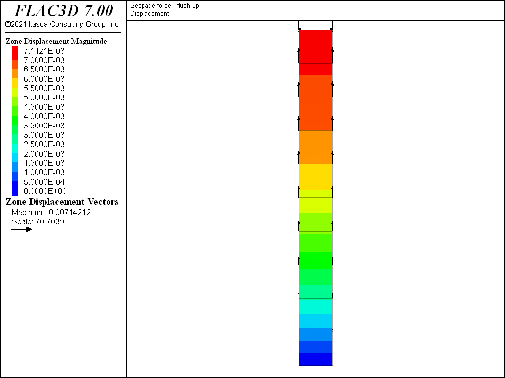
Figure 5: Heave of the layer at steady state — seepage force from over-pressured aquifer.
The analytical solution for the heave can be calculated from Equation (7). There is no change in total stress, and so the term \(\Delta \sigma_{zz}\) drops out. Also, the Biot coefficient is equal to unity. Thus we can write
where \(p^{(3)}\) is given by Equation (17), and \(p^{(4)}\) is the steady-state pore pressure distribution at the end of this stage. This pore pressure is given by
where \(p_b^{(4)}\) = 0.5 MPa. Substitution of Equation (19) and Equation (17) into Equation (18), and further integration produces
For \(y\) = \(H\), we obtain
The FLAC3D result for surface heave compares directly to this result (\(u\) = 7.143 × 10⁻³ m).
Seepage Force (Downwards Flow) — The seepage force case is repeated for the scenario in which the base of the layer is in contact with a high-permeability under-pressured aquifer. This time, a pressure value of \(p_b^{(5)}\) = 0.1 MPa is specified at the base. The displacements are reset, and the coupled calculation is made. The layer settles in this case, which can be seen from the displacement vector plot in Figure 6. The analytical value for the displacement may be derived from Equation (21) after replacing \(p_b^{(5)}\) for \(p_b^{(4)}\). The FLAC3D settlement compares well with the analytical settlement of \(u\) = -7.143 × 10⁻³ m.
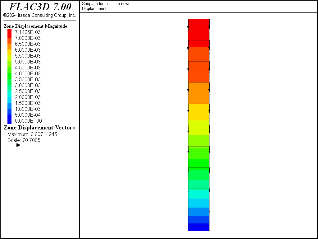
Figure 6: Settlement of the layer at steady state — seepage force from under-pressured aquifer.
The corresponding project file, “WeightBuoyancySeepage.prj,” is located in the “datafiles\fluid\WeightBuoyancySeepage” folder. Below is the datafile.
WeightBuoyancySeepage.dat:
;; Solid weight, buoyancy and seepage forces
model new
model title 'Buoyancy - fully coupled'
model large-strain off
fish automatic-create off
model configure fluid
program call 'fishFunctions'
[setup]
zone create brick size 1 1 10
zone cmodel assign elastic
zone fluid cmodel assign isotropic
zone property bulk [m_bu] shear [m_sh]
zone initialize density [m_d]
; --- (column is dry) ---
zone gridpoint initialize saturation 0
; --- boundary conditions ---
zone face apply velocity-x 0 range union position-x 0 position-x 1
zone face apply velocity-y 0 range union position-y 0 position-y 1
zone face apply velocity-z 0 range position-z 0
; --- gravity ---
model gravity 0 0 [mgrav]
; --- histories ---
fish history num_dis
fish history ana_dis1
; --- initial equilibrium
model fluid active off
model fluid mechanical on
model solve
fish list [num_dis] [ana_dis1]
model save 'ini'

; --- Fully coupled ---
model restore 'ini'
model title 'Buoyancy - fully coupled'
zone gridpoint initialize displacement (0,0,0)
history delete
; --- histories ---
fish history num_dis
fish history ana_dis2
model history fluid time-total
; --- add water ---
zone initialize fluid-density=[w_d]
zone gridpoint initialize saturation 1
zone gridpoint initialize fluid-modulus=2e8
zone gridpoint initialize fluid-tension=-1e10
zone fluid property porosity=[m_n] permeability 1e-8
; --- boundary conditions ---
zone gridpoint fix pore-pressure 0 range position-z 10
; --- static equilibrium ---
model fluid active on
model mechanical active on
model mechanical substep 10
model mechanical slave
model fluid substep 256
; --- we can run this simulation coupled, using ---
model solve fluid time-total 300 or mechanical ratio 1e-6
fish list [num_dis] [ana_dis2]
model save 'ex1a'

; --- Uncoupled ---
model restore 'ini'
model title 'Buoyancy - uncoupled'
zone gridpoint initialize displacement (0,0,0)
history delete
; --- add water ---
zone gridpoint initialize saturation 1
zone initialize fluid-density=[w_d]
zone gridpoint initialize fluid-modulus=2e8
zone gridpoint initialize fluid-tension=-1e10
zone fluid property porosity=[m_n] permeability 1e-8
; --- boundary conditions ---
zone gridpoint fix pore-pressure 0 range position-z 10
; --- static equilibrium ---
model fluid active on
model mechanical active off
; --- we can run this simulation uncoupled, using ---
model solve fluid time-total 300
; --- histories ---
fish history num_dis
fish history ana_dis2

model fluid active off
model mechanical active on
zone gridpoint initialize fluid-modulus 0
model solve ratio 1e-6
fish list [num_dis] [ana_dis2]
model save 'ex1b'

; --- Sink it deeper, under 20m of water ---
model restore 'ex1b'
zone gridpoint initialize fluid-modulus 2e8
model title 'Sink it deeper, under 20m of water'
zone gridpoint initialize displacement (0,0,0)
history delete
; --- fluid boundary conditions ---
zone gridpoint fix pore-pressure 2e5 range position-z 10
; --- apply pressure of water ---
zone face apply stress-normal -2e5 range position-z 10
; --- static equilibrium ---
; --- we can run this simulation uncoupled, using ---
model fluid active on
model mechanical active off
model solve fluid time-total 600
; --- histories ---
fish history num_dis
fish history ana_dis3
model fluid active off
model mechanical active on
zone gridpoint initialize fluid-modulus 0
model solve ratio 1e-6
fish list [num_dis] [ana_dis3]
model save 'ex1c'

; --- Seepage force: flush up ---
model restore 'ex1c'
zone gridpoint initialize fluid-modulus 2e8
model title 'Seepage force:  flush up'
zone gridpoint initialize displacement (0,0,0)
history delete
; --- flush fluid up ---
zone gridpoint fix pore-pressure 5e5 range position-z 0
; --- static equilibrium ---
; --- we can run this simulation uncoupled, using ---
model fluid active on
model mechanical active off
model solve fluid time-total 1200
; --- histories ---
fish history num_dis
fish history ana_dis4
model fluid active off
model mechanical active on
zone gridpoint initialize fluid-modulus 0
model solve ratio 1e-6
fish list [num_dis] [ana_dis4]
model save 'ex1e'

; --- Seepage force: flush down ---
model restore 'ex1c'
zone gridpoint initialize fluid-modulus 2e8
model title 'Seepage force:  flush down'
zone gridpoint initialize displacement (0,0,0)
history delete
; --- flush fluid up ---
zone gridpoint fix pore-pressure 1e5 range position-z 0
; --- static equilibrium ---
; --- we can run this simulation uncoupled, using ---
model fluid active on
model mechanical active off
model solve fluid time-total 1200
; --- histories ---
fish history num_dis
fish history ana_dis5
model fluid active off
model mechanical active on
zone gridpoint initialize fluid-modulus 0
model solve ratio 1e-6
fish list [num_dis] [ana_dis5]
model save 'ex1f'
Pore Pressure Initialization and Deformation
In FLAC3D, when equilibrium stresses are initialized in the model with the zone initialize command
(following, for example, the procedure as described in Stresses with Gradients — Uniform Material
and mechanical steps are taken, no stress increment is calculated by the code,
and thus no displacement is generated, because the model is in equilibrium with the stress boundary conditions and applied loads.
In other words, FLAC3D does not calculate the deformations associated with installation of equilibrium stresses,
when using the zone initialize stress command.
If the stress state is installed in this way at the beginning of a run, the initial stress state is taken as the reference state for displacements.
(This is worth noting because the logic may be different from other codes,
in which the zero stress state is taken as reference for calculation of displacements.)
The situation regarding pore pressure in a fluid-mechanical simulation is similar:
by default, if pore pressures are initialized with the zone gridpoint initialize pore-pressure command,
are in equilibrium with the fluid boundary conditions and hydraulic loading, and fluid steps are taken,
then by default no increment of pore pressure will be generated by the code.
If the zone gridpoint initialize pore-pressure command is issued at the beginning of the run,
this initial state is taken as the reference state for pore pressure.
There will be no stress change (and, if mechanical steps are taken, no displacement)
as a result of the pore pressure initialization,
because no increment of pore pressure is calculated by the code.
In other words, by default, FLAC3D does not calculate the deformation associated with installation of equilibrium pore pressures
when using the zone gridpoint initialize pore-pressure command.
This only applies, by default, to equilibrium pore pressures established using
the zone gridpoint initialize pore-pressure command,
the zone water command or
a FISH function to initialize pore pressures.
Pore pressure change that is calculated by FLAC3D on the other hand,
will always generate stress change;
if the system is brought out of equilibrium by the stress change and mechanical steps are taken,
then deformations will be generated, if conditions allow.
If the deformation associated with a new distribution of pore pressure, assigned using
the zone gridpoint initialize pore-pressure command,
the zone water command or
a FISH function to initialize pore pressures, needs to be calculated,
then a special stress-correction technique needs to be used.
This technique consists of
1) subtracting from the total normal stresses, the increment of pore pressure in the zones affected by the change,
multiplied by Biot coefficient (the pore pressure increment in a zone is calculated by averaging nodal values),
2) adjusting the saturation to zero in the dry region, and to one in the region filled with fluid,
3) adjusting the input material density to the bulk value, above and below the phreatic surface (in case it exists),
and the simulation is run using model configure fluid, and
4) cycling the model to mechanical equilibrium.
A simple example illustrating the heave of a soil layer using this technique is presented below.
Heave of a Soil Layer
For the example, we consider a layer of soil of large lateral extent, and thickness \(H\) = 10 meters, resting on a rigid base. The layer is elastic, the drained bulk modulus, \(K\), is 100 MPa, and the shear modulus, \(G\), is 30 MPa. The bulk density of the dry soil, \(\rho\), is 1800 kg/m3, and the density of water, \(\rho_w\), is 1000 kg/m3. The porosity, \(n\), is uniform; the value is 0.5. And gravity is set to 10 m/sec2.
Initially, the water table is at the bottom of the layer, and the layer is in equilibrium under gravity.
We evaluate the heave of the layer when the water level is raised to the soil surface.
This simple problem is similar to the one analyzed in teh section on Solid Weight, Buoyancy and Seepage Forces.
The difference is, here, we do not require the code to find the new pore-pressure distribution.
The simulation can be carried out with or without using the groundwater configuration (model configure fluid).
We consider both cases.
The grid for this example contains 20 zones: 10 in the \(z\)-direction, 2 in the \(x\)-direction, and 1 in the \(y\)-direction. The origin of axes is at the bottom of the model. The mechanical boundary conditions correspond to roller boundaries at the base and lateral sides of the model.
We first consider equilibrium of the dry layer.
We initialize the stresses, using the zone initialize stress-xx, zone initialize stress-yy and zone initialize stress-zz commands,
using a value of 0.5714 (equal to (\(K-2G/3\))/(\(K+4G/3\))) for the coefficient of earth pressure at rest, \(k_o\).
There are two competing effects on deformation associated with raising the water level: first, the increase of pore pressure will generate heave of the layer; and second, the increase in soil bulk density due to the presence of the water in the pores will induce settlement. To model the combined effects on deformation, of a rise in water level up to the soil surface, we proceed as follows.
If we do not use model configure fluid,
we specify a hydrostatic pore-pressure distribution corresponding to the new water level
by using either the zone gridpoint initialize pore-pressure command or the zone water command,
and we specify a wet bulk density for the soil beneath the new water level.
We apply the stress correction described under point 1) above,
using the commands
zone initialize stress-xx -1e5 add grad 0 0 1e4
zone initialize stress-yy -1e5 add grad 0 0 1e4
zone initialize stress-zz -1e5 add grad 0 0 1e4
Finally, we cycle the model to static equilibrium.
If we do use model configure fluid,
we again specify a hydrostatic pore-pressure distribution corresponding to the new water level
using the zone gridpoint initialize pore-pressure or zone water command.
The saturation is initialized to 1 below the water level, and to zero above.
However, we do not update the soil density to account for the presence of water beneath the new water level (this is done automatically by the code).
We again perform a stress correction, as described earlier.
Finally, we model fluid active off and cycle the model to static equilibrium.
The final response is identical for both cases. The plot of displacement vectors in Figure 7 indicates that the rise of the water table has induced a heave of the soil layer. The surface heave, \(u_h\), can be evaluated analytically using Equation (22),
where \(\alpha_1 = K + 4G/3\). The theoretical value for \(u_h\) is 1.786 × 10⁻³ meters. The theoretical and numerical values compare well. The data files for the simulations are listed in SoilLayerHeave-NoFluid.dat and SoilLayerHeave-withFluid.dat.
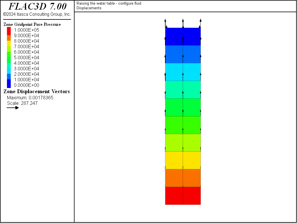
Figure 7: Heave of a soil layer.
SoilLayerHeave-NoFluid.dat:
model new
model large-strain off
model title 'Raising the water table - not in configure fluid'
fish automatic-create off
program call 'fishFunctions'
[setup]
zone create brick point 0 (0,0,0) point 1 (2,0,0) point 2 (0,1,0) ...
                  point 3 (0,0,10) size 2 1 10 ratio 1 1 1
zone cmodel assign elastic
zone property bulk [m_bu] sh [m_sh]
; --- column is dry ---
zone property density [m_d]
; --- boundary conditions ---
zone face apply velocity-z 0 range position-z 0
zone face apply velocity-x 0 range union position-x 0 position-x 2
zone face apply velocity-y 0 range union position-y 0 position-y 1
; --- gravity ---
model gravity 0 0 [mgrav]
; --- histories ---
history interval 10
zone history displacement-z position (0,0,10)
fish history ana_dis
; --- initial equilibrium ---
zone initialize stress-zz -1.8e5   grad 0 0 1.8e4
zone initialize stress-xx -1.029e5 grad 0 0 1.029e4
zone initialize stress-yy -1.029e5 grad 0 0 1.029e4
model solve ratio 1e-6
model save 'ini'
; --- raise water level ---
; (note: when not in configure FLUID, water density is assigned using:)
zone water density [w_d]
; (we can do it this way ...)
zone gridpoint initialize pore-pressure 1e5 grad 0 0 -1e4
; (or this way ...)
;water table origin 0 0 _H normal 0 0 -1
; (total stress adjustement)
zone initialize stress-xx -1e5 add grad 0 0 1e4
zone initialize stress-yy -1e5 add grad 0 0 1e4
zone initialize stress-zz -1e5 add grad 0 0 1e4
; --- use wet density below water table ---
zone property density [m_rho]
; --- static equilibrium ---
model solve ratio 1e-6
model save 'ncfl'
SoilLayerHeave-withFluid.dat:
model new
model title 'Raising the water table - configure fluid'
model large-strain off
fish automatic-create off
model configure fluid
program call 'fishFunctions'
[setup]
zone create brick point 0 (0,0,0) point 1 (2,0,0) point 2 (0,1,0) ...
                  point 3 (0,0,10) size 2 1 10 ratio 1 1 1
zone cmodel assign elastic
zone fluid cmodel assign isotropic
zone property bulk [m_bu] sh [m_sh]
; --- column is dry ---
; (initialize sat at 0)
zone gridpoint initialize saturation 0
zone property density [m_d]
; --- boundary conditions ---
zone face apply velocity-z 0 range position-z 0
zone face apply velocity-x 0 range union position-x 0 position-x 2
zone face apply velocity-y 0 range union position-y 0 position-y 1
; --- gravity ---
model gravity 0 0 [mgrav]
; --- histories ---
history interval 10
zone history displacement-z position (0,0,10)
fish history ana_dis
; --- initial equilibrium ---
zone initialize stress-zz -1.8e5   grad 0 0 1.8e4
zone initialize stress-xx -1.029e5 grad 0 0 1.029e4
zone initialize stress-yy -1.029e5 grad 0 0 1.029e4
;
model fluid active off
model mechanical active on
zone gridpoint initialize fluid-modulus 0
model solve
model save 'ini'
; --- raise water level ---
; (initialize sat at 1 below the water level)
zone gridpoint initialize saturation 1
; (note: in configure FLUID, water density is assigned using:)
zone initialize fluid-density [w_d]
; (we can do it this way ...)
zone gridpoint initialize pore-pressure 1e5 grad 0 0 -1e4
; (or this way ...)
; (note: we can use water table command in configure fluid,
;  this is different from FLAC)
;water table origin 0 0 _H normal 0 0 -1
; (total stress adjustement)
zone initialize stress-xx -1e5 add grad 0 0 1e4
zone initialize stress-yy -1e5 add grad 0 0 1e4
zone initialize stress-zz -1e5 add grad 0 0 1e4
; --- Note:  no need to specify wet density below water table ---
; --- static equilibrium ---
model fluid active off mech on
zone gridpoint initialize fluid-modulus 0
model solve
model save 'cfl'
Effect of the Biot Coefficient
The Biot coefficient, \(\alpha\), relates the compressibility of the grains to that of the drained bulk material:
where \(K\) is the drained bulk modulus of the matrix, and \(K_s\) is the bulk modulus of the grains (see Detournay and Cheng 1993, for reference).
For soils, matrix compliance is usually much higher than grain compliance (i.e., \(1/K >>> 1/K_s\)), and it is a valid approximation to assume that the Biot coefficient is equal to 1.
For porous rocks, however, matrix and rock compliances are most often of the same order of magnitude and, as a result, the Biot coefficient may be almost zero. Consider, for example, a sample of porous elastic rock. The pores are saturated with fluid at a pressure, \(p\), and a total external pressure, \(P\), is applied around the periphery (i.e., on the outside of an impermeable sleeve). The problem can be analyzed by superposition of two stress states: state a, in which fluid pressure and external pressure are both equal to \(p\); and state b, in which pore pressure is zero, and the external pressure is \(P - p\) (see Figure 8).
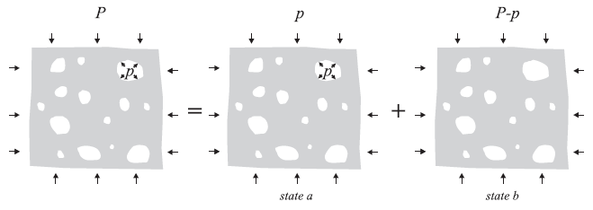
Figure 8: Decomposition of stresses acting on a porous, elastic rock.
The stress-strain relation for state a may be expressed as
For state b (there is no fluid), we can write
The total strain is given by superposition of the strain in state a and in state b:
After substitution of \(\epsilon_a\) from Equation (24), and \(\epsilon_b\) from Equation (26), we obtain
After some manipulations, the stress-strain equation takes the form
Clearly, then, in the framework of Biot theory, a zero Biot coefficient implies that the elastic stress-strain law becomes independent of pore pressure. Of course, in general, porous rocks do not behave elastically, and pore pressure has an effect on failure. Also, if fluid flow in rocks occurs mainly in fractures, Biot theory may not be applicable. Nonetheless, there are numerous instances where the small value of the Biot coefficient may help explain why pore pressure has little effect on deformation for solid, porous (i.e., unfractured) rocks. (For example, the effect on surface settlement of the raising or lowering of the water table in a solid porous rock mass may be unnoticeable.)
Note that the preceding discussion addresses only one of the effects of grain compressibility. The Biot coefficient also enters the fluid constitutive law, which relates change of fluid content to volumetric strain.
The logic for grain compressibility, as developed in the framework of Biot theory, is provided in FLAC3D. Simple verification examples are described below to illustrate the logic.
For reference, in the examples below, in the special case \(\Delta \epsilon_{yy}\) = 0, the principal stress-strain relations have the form
where \(\Delta \xi\) is the variation of fluid content per unit volume of porous media, and \(\Delta \epsilon_v\) is the incremental volumetric strain.
Undrained Oedometer Test
An undrained oedometer test is conducted on a saturated poro-elastic sample.
The Biot modulus is 1 MPa, and the Biot coefficient is 0.3 for this test.
The model is a single square zone of unit dimensions with roller boundaries on the sides and bottom.
A constant velocity, \(v\), is applied to the top.
Fluid flow is turned off, and the simulation is run for 10 calculational steps.
The zone fluid biot on command is given to select the Biot modulus and coefficient rather than the fluid bulk modulus.
Because the sample is laterally confined, \(\Delta \epsilon_{xx}\) = \(\Delta \epsilon_{yy}\) = 0 and \(\Delta \epsilon_v = \Delta \epsilon_{zz}\). For undrained conditions, \(\Delta \xi\) = 0. The analytical value for pore pressure (see Equation (31)) is then
The analytical stresses are obtained by substituting pore pressure and strain components into Equation (29) and Equation (30):
After 10 calculation steps, \(\Delta \epsilon_{zz} = -10v\). The agreement between analytical and numerical values for pore pressure and stresses is checked with the FISH function checkit. The analytical and numerical results are identical. The corresponding project file, “UndrainedOedometer.prj”, is located in the “datafiles\Fluid\UndrainedOedometer” folder. Below is the datafile:
UndrainedOedometer.dat:
; Undrained Oedometer Test
model new
model title 'Undrained Oedometer test'
model large-strain off
fish automatic-create off
model configure fluid
zone create brick point 0 (0,0,0) point 1 (1,0,0) ...
                  point 2 (0,1,0) point 3 (0,0,1) size 1 1 1
zone cmodel assign elastic
zone fluid cmodel assign isotropic
zone property bulk 1e8 shear 0.3e8
zone gridpoint initialize fluid-tension -1e10
zone fluid biot on
zone fluid property porosity=0.5 biot=0.3
; --- boundary conditions ---
zone gridpoint fix velocity
zone gridpoint initialize velocity-z=-1e-3 range position-z 1
; --- undrained compression ---
zone gridpoint initialize biot=1e8
model fluid active off
model mechanical active on
model step 10
Pore Pressure Generation in a Confined Sample
The effect of pore pressure generation is shown for the case of a confined sample in an impermeable sleeve. The sample geometry and properties are the same as in the previous example, Undrained Oedometer Test. Roller boundaries are set on all four sides of the model. The boundaries are also impermeable (by default). Fluid flow is turned on, and a volumetric water source with a unit flow rate is applied to the model to raise the pore pressure. The simulation is run for 10 fluid flow steps.
At the end of the simulation, \(\Delta \xi = 10\Delta t\). The grid is fully constrained, hence \(\Delta \epsilon_{xx} = \Delta \epsilon_{yy} = \Delta \epsilon_{zz} = \Delta \epsilon_v = 0\). The analytical value for pore pressure is found, from Equation (31), to be
The analytical stresses are then derived from Equation (29) and Equation (30) to be
Numerical and analytical values for pore pressure and stresses are compared with the FISH function checkit, and the results are identical. The corresponding project file, “PorePressureGenerationConfined.prj” is located in the “datafiles\Fluid\PorePressureGenerationConfined” folder. Below is the data file:
PorePressureGenerationconfined.dat:
; file for 'Pore pressure generation in a confined sample'
model new
model title 'Pore pressure generation in a confined sample'
fish automatic-create off
model configure fluid
zone create brick point 0 (0,0,0) point 1 (1,0,0) point 2 (0,1,0) ...
                  point 3 (0,0,1) size 1 1 1
zone cmodel assign elastic
zone fluid cmodel assign isotropic
zone property bulk 1e8 shear 0.3e8
zone gridpoint initialize fluid-tension -1e10
zone fluid biot on
zone fluid property porosity=0.5 biot=0.3 permeability=1e-10
zone gridpoint initialize biot=1e8
; --- boundary conditions ---
zone gridpoint fix velocity
; --- water source ---
zone apply well 1.0
model fluid active on
model mechanical active off
model step 10
Pore Pressure Generation in an Infinite Layer
This example is similar to the preceding confined sample, except that the top boundary is not constrained. All boundaries are impermeable, and a volumetric water source with unit flow is applied to raise the pore pressure. Both mechanical and fluid-flow calculations are turned on, and the simulation is run for 10 fluid-flow steps. Note that 200 mechanical sub-steps are taken every fluid step in order to keep the system in quasi-static equilibrium state.
For this example, \(\Delta \epsilon_{xx} = \Delta \epsilon_{yy} = 0\), \(\Delta \epsilon_v = \Delta \epsilon_{zz}\) and \(\Delta \sigma_{zz} = 0\). Using these conditions in Equation (30), we obtain
After substituting Equation (37) for \(\Delta p\) in Equation (31) and solving for \(\epsilon_{zz}\), we find
Analytical expressions for pore pressure and stress can now be derived from Equation (29) and Equation (31):
Numerical and analytical values for vertical displacement, pore pressure and stresses are compared with the FISH function checkit, and the results are identical. The corresponding project file, “PorePressureGenerationInfinite.prj” is located in the “datafiles\Fluid\PorePressureGenerationInfinite” folder. Below is the data file:
PorePressureGenerationinfinite.dat:
; file for 'Pore pressure generation in an infinite layer'
model new
model large-strain off
model title 'Pore pressure generation in an infinite layer'
fish automatic-create off
model configure fluid
zone create brick point 0 (0,0,0) point 1 (1,0,0) point 2 (0,1,0) ...
                  point 3 (0,0,1) size 1 1 1
zone cmodel assign elastic
zone fluid cmodel assign isotropic
zone property bulk 2.0 shear 1.0
zone gridpoint initialize fluid-tension -1e10
zone fluid biot on
zone fluid property porosity=0.5 biot=0.3 permeability=1.0
zone gridpoint initialize biot=1
; --- boundary conditions ---
zone gridpoint fix velocity-x
zone gridpoint fix velocity-y
zone gridpoint fix velocity-z range position-z 0
; --- water source ---
zone apply well 1.0
model fluid active on
model mechanical active on
model fluid substep 1
model mechanical substep 200
model mechanical slave
model solve fluid time-total 1.6 or mechanical ratio 1e-10
;
model save 'ppgen-infinite'
| Was this helpful? ... | FLAC3D © 2019, Itasca | Updated: Feb 25, 2024 |