FLAC3D Theory and Background • Constitutive Models

Cap-Yield (CYSoil) Model*

Note

*Not available in 3DEC.

The CYSoil model is a strain-hardening constitutive model characterized by a frictional and cohesive Mohr-Coulomb shear envelope and an elliptic volumetric cap with ratio of axes, defined by a shape parameter \(\alpha\). The CYSoil model in FLAC3D 6 is an updated version of the FLAC3D 5 CYSoil model with the following built-in features:

• a cap hardening law to capture the volumetric power law behavior observed in isotropic compaction tests;

• a friction-hardening law to reproduce the hyperbolic stress-strain law behavior observed in drained triaxial tests; and

• a compaction/dilation law to model irrecoverable volumetric strain taking place as a result of soil shearing.

The motivation for closing the yield surface by a cap on the mean stress axis is to permit plastic behavior in response to an isotropic stress increase. This plasticity effect accounts for grain crushing and rearrangement, and is particular to soils. In the double-yield model, the cap is a plane, normal to the mean stress axis in stress space. The impact of this particular shape on the coefficient of lateral earth pressure, \(K_0\), as predicted by the model in uniaxial compression tests, has been considered to be somewhat restrictive by some users. In that respect, the CYSoil model is a modification of the double-yield model that addresses this issue by accounting for a cap with an elliptic shape in the (\(p^{\prime}\), \(q\)) plane. The ratio of axes of the ellipse, \(\alpha\), determines the value of \(K_0\) and is a material property for the model, which can be chosen to match a known value in uniaxial compression. In particular, a planar volumetric cap is obtained as a special case of the CYSoil formulation by assuming a value \(\alpha \gg 1\).

In addition, when subjected to deviatoric loading, soils usually exhibit a decrease in stiffness, accompanied by irreversible deformation. In most cases, the plot of deviatoric stress versus axial strain obtained in a drained triaxial test may be approximated by a hyperbola. This feature has been used by Duncan and Chang (1970) to formulate their well-known “hyperbolic soil” model. The hyperbolic soil model of Duncan and Chang is a nonlinear elastic model that has been shown to exhibit some drawbacks. These drawbacks include, for example, difficulty in detecting and characterizing unloading/reloading and,in specific cases, producing a nonphysical bulk-modulus value that can lead to an erroneous energy generation in the model. Because the CYSoil model is formulated in the theory of hardening plasticity, it allows for an alternative expression of the hyperbolic behavior (based on friction hardening), which is capable of addressing some of these problems. A simplified version of the CYSoil model, called the CHSoil model, also addresses the difficulties of the Duncan and Chang model and is provided as an alternative to the Duncan and Chang model.

When tested under drained triaxial conditions, soils generally exhibit shear-induced volume changes that are strongly dependent on soil density. Typically, there is a tendency for the soil to contract under small shear strains, and to dilate under larger strains, unless it is very loose (Byrne et al. 2003). In particular, when fluid fills the pores, it is this tendency of the soil skeleton to contract and dilate that controls its liquefaction response. Also, the shear-stress/shear-strain response of loose soil may exhibit a softening response under undrained conditions. It is the existence of a peak in shear strength which may lead to instability (static liquefaction) during a monotonic load-controlled process (Boukpeti 2001). Shear-induced volume changes can be accounted for in the CYSoil model by means of a dilation hardening/softening law.

Formulations

In this section, principal stress, \(\sigma_i\), and strain, \(e_i\), i = 1,3, components are positive in tension. Also, all stresses are effective by default if not explicitly stated. The principal effective stresses are with the order \(\sigma_1 \le \sigma_2 \le \sigma_3\), and \(\sigma_1\) is the most compressive stress.

Incremental Elastic Law

The elastic behavior is expressed using Hooke’s law. The incremental expression of the law in terms of principal stress and strain has the form

(1)\[\begin{split}\begin{matrix} \Delta \sigma_1 = \alpha_1 \Delta e_1^e + \alpha_2 (\Delta e_2^e + \Delta e_3^e) \\ \\ \Delta \sigma_2 = \alpha_1 \Delta e_2^e + \alpha_2 (\Delta e_1^e + \Delta e_3^e) \\ \\ \Delta \sigma_3 = \alpha_1 \Delta e_3^e + \alpha_2 (\Delta e_1^e + \Delta e_2^e) \end{matrix}\end{split}\]

where \(\alpha_1 = K^e + 4G^e / 3\), \(\alpha_2 = K^e - 2G^e / 3\), and \(K^e\) and \(G^e\) are current, tangent elastic bulk and shear modulus, respectively.

In the constitutive model logic, the modulus \(G^e\) is related to the mean effective pressure by a power law. The user provides the value of Poisson ratio \(\nu\), which is assumed to remain constant. In addition, the user can provide upper and lower bound values for \(G^e\), which will then overwrite the default settings for these parameters. Note that the upper bound for \(G^e\) is used for numerical stability: a value close to the maximum value reached during the simulation should be assigned to the parameter; if a much larger value is assigned, the numerical convergence may be slow.

The bulk modulus \(K^e\) is derived internally, using the relation:

(2)\[ K^e = G^e {{2(1 + \nu)} \over {3 (1 - 2\nu)}}\]

Yield and Potential Functions

Shear Yield Criterion and Flow Rule

Shear yielding is defined by a Mohr-Coulomb criterion (see representation in Figure 1):

(3)\[ f^s = \sigma_1 - N_m \sigma_3 + 2c_m\sqrt{N_m}\]

where \(N_m = (1 + \sin \phi_m) / (1 - \sin \phi_m)\), \(\phi_m\) is the mobilized friction, a quantity which can increase between an initial value (possibly zero), and a final value \(\phi_f\) set by the user.

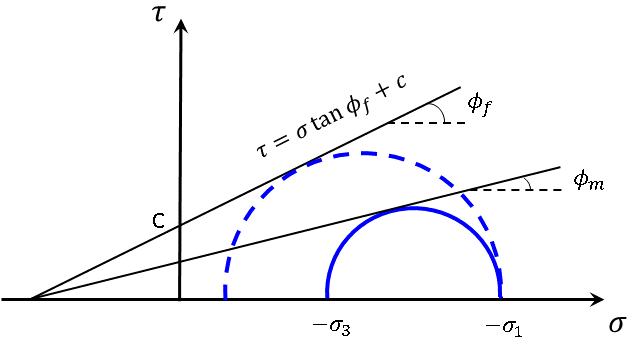
Figure 1: Mohr circles at in-situ stress and at failure.

Note that in the model logic, unloading is elastic, and thus \(\phi_m\) cannot decrease. The last term of Equation (3) contains mobilized cohesion, \(c_m\), which can increase between an initial value and an ultimate value, \(c\), defined by the user. The expression for \(c_m\) is:

(4)\[ c_m = c {{\tan \phi_m} \over {\tan \phi_f}}\]

The shear yield envelope (see Equation (3)) can also be expressed in an alternative form (consistent with the cap formulation) as follows:

(5)\[ f^s = M (p + c\cot \phi_f) - q\]

where \(M = 6 \sin \phi_m / (3 - \sin \phi_m)\), \(p\) is the mean effective stress, \(p\) = -(\(\sigma_1\) + \(\sigma_2\) + \(\sigma_3\))/3, and \(q\) is a measure of shear stress, defined as \(q = - [\sigma_1 + (\delta - 1)\sigma_2 - \delta \sigma_3]\), where \(\delta = (3+\sin \phi_m) / (3-\sin \phi_m)\).

The potential function is nonassociated and has the form

(6)\[ g^s = M^* p - q^*\]

where \(q^* = -[\sigma_1 + (\delta^* - 1)\sigma_2 - \delta^* \sigma_3]\), \(\delta^* = (3+\sin \psi_m) / (3-\sin \psi_m)\), \(M^* = 6 \sin \psi_m / (3 - \sin \psi_m)\), and \(\psi_m\) is the mobilized dilatancy angle.

Volumetric Cap Criterion and Flow Rule

Yielding on the cap is associated with the criterion:

(7)\[ f^c = g^c = {q^2 \over \alpha^2} + p^2 - p^2_c\]

where \(\alpha\) is a dimensionless parameter, defining the shape of the elliptical cap in the (\(p\), \(q\)) plane, and \(p_c\) is the current cap pressure. Note that the ellipsoid degenerates into a spherical cap for \(\alpha = 1\) (default setting), and to a planar volume cap for \(\alpha \gg 1\).

Tensile Yield Criterion and Flow Rule

The tensile yield function is the same as that used for the Mohr-Coulomb model:

(8)\[ f^t = g^t = \sigma^t - \sigma_3\]

where \(\sigma^t\) is the tensile strength. The potential function for tensile yielding is associated.

Built-in Hardening Functions

Cap Hardening

Soil stiffness usually increases in a nonlinear fashion as a function of isotropic pressure. In the CYSoil model, soil volumetric behavior in an isotropic compaction test is described by the following power law:

(9)\[ {{dp} \over {de}} = K_{ref} p_{ref} \left({{p} \over {p_{ref}}}\right)^m\]

where \(e\) is the volumetric strain taken positive in compression, \(K_{ref}\) is the tangent elastic bulk modulus number, the product \(K_{ref}p_{ref}\) is the slope of the laboratory curve for \(p\) versus \(e\) at reference effective pressure, \(p_{ref}\), and \(e\) is a constant ( \(0 < m < 1\)).

A typical graph, representative of this law, is sketched with a small unloading excursion in Figure 2. The equation for the curve (obtained by integration of Equation (9) and using \(p = 0\) at \(e = 0\) is:

(10)\[ p = K_{ref} \left[ (1-m) K_{ref} e \right]^{{1} \over {1-m}}\]

The usual assumption is made that the total strain increment is the sum of the elastic and plastic contributions:

(11)\[ de = de^e + de^p\]

In this context, \(e^p\) is the plastic volumetric strain contribution from cap yielding only, not including shear yielding.

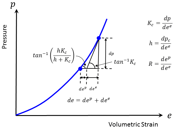
Figure 2: Isotropic consolidation test: pressure versus volumetric strain.

Also, the tangent elastic modulus, \(K^e\), and plastic modulus, \(H\) are defined as follows:

(12)\[K^e = {{dp} \over {de}}\]

(13)\[H = {{dp_c} \over {de^p}}\]

As the material becomes more compact, its plastic stiffness usually increases; it seems reasonable that the elastic stiffness will also increase, since the grains are being forced closer together. The CYSoil model uses a simple rule whereby under general loading conditions, the current elastic modulus is equal to a constant, \(R\) times the current plastic modulus:

(14)\[K^e = RH\]

Substitution of H from Equation (13) in Equation (14) gives:

(15)\[K^e = R {{dp_c} \over {de}} {{de} \over {de^p}}\]

Using Equation (11) in Equation (15), we obtain

(16)\[K^e = R {{dp_c} \over {de}} \left( 1 + {{de^e} \over {de^p}} \right)\]

For isotropic compression, \(dp = dp_c\) and by definition of \(K^e\) and \(H\) (see Equations (12) and (13)), it follows from Equation (14) that

(17)\[R = {{de^p} \over {de^e}}\]

Now, substituting Equation (16) into Equation (15), one obtains

(18)\[K^e = (1 + R) {{dp_c} \over {de}}\]

Thus, using the definition (Equation (9)) for \(dp_c / de\) in Equation (18), the tangent elastic bulk modulus, \(K^e\) is dependent on cap pressure, \(p_c\) (or maximum effective pressure sustained by the material in the past), according to the following power law:

(19)\[K^e = (1 + R) K_{ref} p_{ref} \left({{p_c} \over {p_{ref}}}\right)^m\]

According to Equations (9) and (18), the tangent elastic shear modulus obeys the following power law:

(20)\[G^e = (1 + R) G_{ref} p_{ref} \left({{p_c} \over {p_{ref}}}\right)^m\]

where

(21)\[G^e_{ref} = K_{ref} {{3(1-2\nu)} \over {2(1+\nu)}}\]

The input parameter \(G_{ref}\), \(p_{ref}\), \(m\), and \(R\) must be provided by the user.

In addition, the user can provide upper and lower bound values for \(G^e\) (\(G^e_{max}\) and \(G^e_{min}\)), which will then overwrite the default settings for these parameters. Note that the upper bound for \(G^e\) is used for numerical stability: a value close to the maximum value reached during the simulation should be assigned to the parameter. If a much larger value is assigned, the numerical convergence may be slow.

After substituting Equation (19) into Equation (14), the expression for the hardening modulus, \(H\), becomes

(22)\[H = {{dp_c} \over {de^p}} = K_{ref} p_{ref} {(1+R) \over R} \left({{p_c} \over {p_{ref}}}\right)^m\]

Integration of Equation (22) for m < 1 by assuming \(p_c\) = 0 at \(e^p\) = 0 provides the evolution law for the cap pressure, \(p_c\), in terms of plastic volumetric strain, \(e^p\):

(23)\[p_c = p_{ref} \left[K_{ref} (1-m) {(1+R) \over R} e^p \right]^{1 \over (1-m)}\]

Conversely, the plastic volumetric strain is expressed in terms of \(p_c\) as:

(24)\[e^p = {1 \over {1-m}} \cdot {R \over {1+R}} \cdot {1 \over K_{ref}} \left({{p_c} \over {p_{ref}}}\right)^{1-m}\]

Note that the code sets an upper bound of 0.99 for \(m\). However, it may be interesting to know that in the limiting case of \(m\) = 1, Equation (22) for m < 1 by assuming \(p_c\) = 0 at \(e^p\) = 0 provides a logarithmic law that is similar to the expression used by the Cam-Clay model:

(25)\[\ln {p_c \over p_{c0}} = {{R+1} \over R} K_{ref} (e^p - e^p_0)\]

Friction Hardening

For most soils, the plot of deviatoric stress versus axial strain obtained in a drained triaxial test can be approximated by a hyperbola (Figure 3). The CYSoil model incorporates a friction-strain hardening law to capture this behavior.

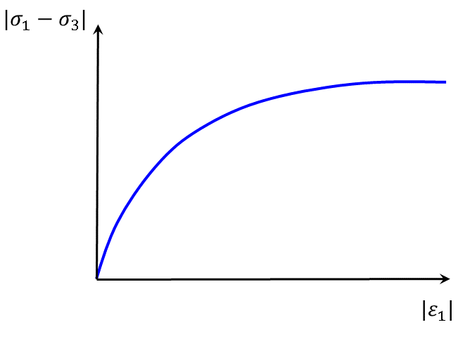
Figure 3: Deviatoric stress versus axial strain for a generic triaxial test.

The evolution parameter for the cap volumetric yielding envelope and that for the shear yielding envelope are independent in the CYSoil model. By convention, the mobilized plastic shear moduli, \(G^p_m\) is defined as:

(26)\[ G^p_m = {d(\sin \phi_m) \over d(\gamma^p)} p_{ref}\]

where \(\phi_m\) is the mobilized friction angle and \(\gamma^p\) is plastic shear strain. Thus, the ratio \(G^p_m/p_{ref}\) is the slope of the curve in a graph of mobilized stress ratio, \(\sin \phi_m\), versus plastic shear strain \(\gamma^p\). The expression for mobilized plastic shear modulus is adopted from Byrne et al. (2003):

(27)\[ G^p_m = G^p_{m,i} \left( 1 - {{\sin \phi_m - \sin \phi_0} \over {\sin \phi_f - \sin \phi_0}} R_f \right)^2\]

In this formula, \(\phi_0\) is an internal constant (which, by default is set equal to the user-provided mobilized friction angle under in-situ conditions), \(\phi_f\) is the ultimate friction angle, \(G^p_{m,i}\) is the value of \(G^p_m\) under in-situ conditions, \(R_f\) is the failure ratio used to assign a lower bound for \(G^p_m\). Note that \(R_f\) < 1, and a typical value used in many cases is \(R_f\) = 0.9.

For the CYSoil model, \(G^p_{m,i}\) is expressed as

(28)\[ G^p_{m,i} = \beta (1+R) G_{ref} p_{ref}\]

where \(beta\) is a user-defined calibration factor, which can depend on the value of confinement (in triaxial test modeling) or in-situ confining stress (in field scale modeling).

After substituting Equations (27) and (28) in Equation (26) and rearranging some terms, we obtain:

(29)\[ d\gamma^p = {1 \over {\beta (1+R) G_{ref}}} \cdot {{d(\sin \phi_m)} \over {\left( 1 - {{\sin \phi_m - \sin \phi_0} \over {\sin \phi_f - \sin \phi_0}} R_f \right)^2}}\]

The evolution law for mobilized friction, \(\phi_m\), in terms of plastic shear strain, \(\gamma^p\), for the CYSoil model is obtained by integration of Equation (27), considering that \(\gamma^p\) = 0 at \(\phi_m = \phi_0\):

(30)\[ \sin \phi_m = \sin \phi_0 + {{\beta \gamma^p (1+R) G_{ref} (\sin \phi_f - \sin \phi_0)} \over {(\sin \phi_f - \sin \phi_0) + \beta \gamma^p (1+R) G_{ref} R_f}}\]

Equation (30) is used in the built-in logic to calculate the mobilized friction from the accumulated plastic shear strain.

Note that after solving Equation (30) for \(\gamma^p\) with \(\phi_0 = 0\), one obtains:

(31)\[ \gamma^p = {{1} \over {\beta(1+R)G_{ref}}} {{\sin \phi_f \sin \phi_m} \over {\sin \phi_f - \sin \phi_m R_f}}\]

The mobilized plastic shear modulus can be expressed in terms of plastic shear strain by substitution of Equation (31) for \(\sin \phi_m\) into Equation (27) and performing some manipulations:

(32)\[ {{G^p_m} \over {G^p_{m,i}}} = \left( 1 \over {1 + A \gamma^p} \right)^2\]

where

(33)\[ A = \beta {{(1+R) G_{ref} R_f} \over {\sin \phi_f - \sin \phi_0}}\]

The graph of \({G^p_m}/{G^p_{m,i}}\) versus \(\log \gamma^p\) is represented in generic form in Figure 4.

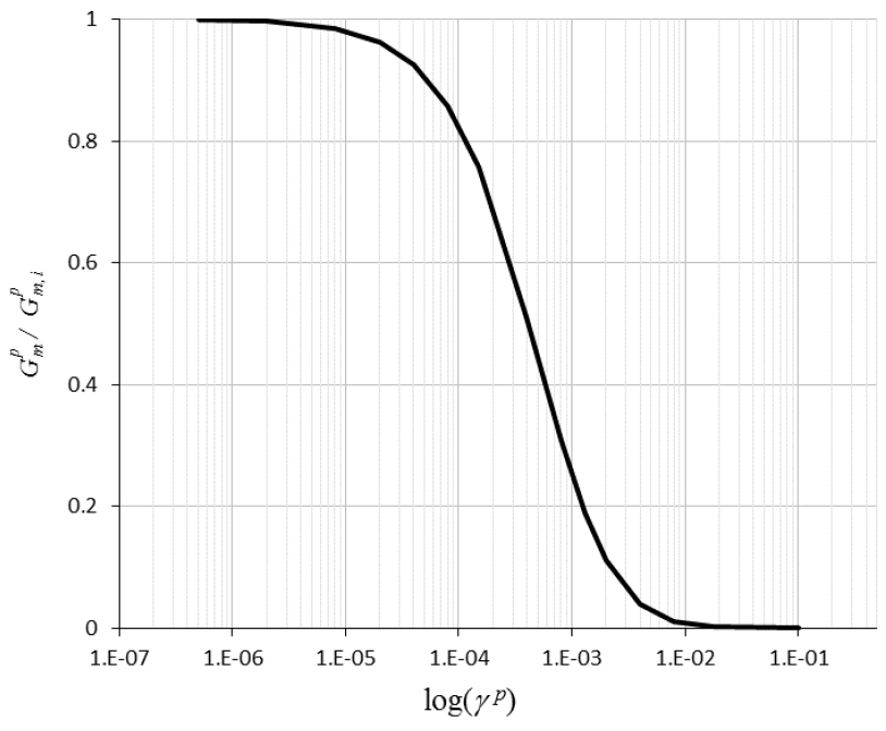
Figure 4: Generic form of plot \({G^p_m}/{G^p_{m,i}}\) versus \(\log \gamma^p\).

It is assumed that the curve at very small strain (see Figure 4) is derived from in-situ conditions (e.g., by using seismic shear wave velocity profiles drawn by cross-hole or down-hole tests), and that \(\gamma^p\) is the plastic shear strain that develops after initial conditions have been established. In this case, the initial value of the evolution parameter \(\gamma^p\) should be left at zero (default value). The code will automatically set the parameter \(\phi_0\) equal to the initial value of mobilized friction, friction mob, provided by the user. The implication is that the graph in Figure 4 will be exercised starting at \(\gamma^p\) = 0 during the simulation.

Alternatively, the user can exercise the modulus degradation curve in a simulation, starting with a value of \(\gamma^p\) that is larger than zero. This option provides additional calibration flexibility. Note that when the initial non-zero value of \(\gamma^p\) is provided by the user, the code automatically sets the internal constant \(\phi_0\) to zero. For example, Equation (31) can be used to derive a value of plastic shear strain, consistent with the user-provided mobilized friction angle, for input into the code.

Dilation Hardening

A certain amount of irrecoverable volumetric strain, \(e^p\), is expected to take place as a result of soil shearing. Also, under small (monotonic or cyclic) shear strains, there is a tendency for the soil skeleton to contract due to grain rearrangements. For larger shear strains, the soil skeleton may dilate if the soil is dense as a result of grains riding over each other. A dilation strain-hardening table is used to model this non-monotonic behavior. For the CYSoil model, the shear-hardening flow rule has the form

(34)\[ {{d e^p_s} \over {d \gamma^p}} = \sin \psi_m\]

where \(\psi_m\) is the mobilized dilation angle. The evolution law for mobilized dilation angle ψm is given by the following law, based on Rowe’s stress-dilatancy theory (1962):

(35)\[ \sin \psi_m = {{\sin \phi_m - \sin \phi_{cv}} \over {1 - \sin \phi_m \sin \phi_{cv}}}\]

where \(\sin \phi_m\) is given in terms of \(\gamma^p\) by Equation (30), and \(\sin \phi_{cv}\) is a constant. According to the law of Equation (35), the material contracts for \(\sin \phi_m < \sin \phi_{cv}\) and dilates for \(\sin \phi_m > \sin \phi_{cv}\). In most cases, the constant volume stress ratio \(\sin \phi_{cv}\) can be expressed in terms of (known) ultimate values of friction, \(\sin \phi_f\) , and dilation, \(\sin \psi_f\) , as follows:

(36)\[ \sin \phi_{cv} = {{\sin \phi_f - \sin \psi_f} \over {1 - \sin \phi_f \sin \psi_f}}\]

and \(\phi_f\) and \(\psi_f\) are ultimate (known) values of friction and dilation, respectively.

Dilatancy Cut-off

In addition, a dilatancy cut-off can be specified whereby the mobilized dilation angle is set to zero when the void ratio, \(\hat{e}\), exceeds a specified value, \(\hat{e}_{max}\). The values of initial (in-situ) void ratio, \(\hat{e}_{ini}\), and final void ratio, \(\hat{e}_{max}\), are provided by the user. The current value of void ratio \(\hat{e}\) is calculated by the code from the known volumetric strain, \(e\) (positive for extension), initial (in-situ) volumetric strain, \(e_{ini}\) (usually zero), and initial void ratio, \(\hat{e}_{ini}\), using

(37)\[ \hat{e} = (1 + \hat{e}_{ini}) \exp (e - e_{ini}) - 1\]

so that \(\psi_m\) = 0 if \(\hat{e} \ge \hat{e}_{max}\).

Choice of Material Parameters

By default, the basic CYSoil model includes the following features and functionalities, as described above:

• A frictional and cohesive strain-hardening Mohr-Coulomb shear envelope together with: 1) a built-in friction-hardening law to reproduce the hyperbolic stress-strain law behavior observed in drained triaxial tests; and 2) a built-in dilation hardening/softening law to model shear-induced volume changes whereby the soil contracts under small shear strains and dilates under larger strains.

• An elliptic volumetric cap with a ratio of axes defined by a shape parameter, which can be chosen to match a known value of lateral earth pressure, in uniaxial compression, combined with a built-in cap hardening law to capture the volumetric power-law behavior observed in isotropic compaction tests.

General guidelines to select the properties for the basic model are provided below.

Initialization of \(G_{ref}\), \(R\) and \(m\)

The “hardening curve” and ratio, \(R\), of elastic bulk modulus to plastic bulk modulus are volumetric properties that may be derived from the results of an isotropic compression test. The laboratory curve, including a small unloading excursion, is sketched in Figure 2. The parameter \(R\) can be estimated from the graph by taking the ratio of the two quantities \(de^p\) and \(de^e\) measured from the unloading excursion (see Equation (17)). The two additional volumetric model parameters \(G_{ref}\) and \(m\) appearing in Equation (10) can be obtained by fitting this equation to the laboratory curve (see sketch in Figure 2). To facilitate the curve fitting process, a first estimate of \(G_{ref}\) can be calculated from Equation (9), using a starting value of \(m\) = 0.5 and the quantities \(dp\) and \(de\) measured on the graph close to the unloading point. Some iterations can then be taken in which \(G_{ref}\) and \(m\) are adjusted to obtain a better fit to the lab curve. In turn, the parameter \(G_{ref}\) can be estimated (from known values of \(K_{ref}\) and \(\nu\)) using Equation (21).

Alternatively, the model parameters \(G_{ref}\) and \(R\) can be estimated from published values of parameters \(E^{ref}_{ur}\) and \(E^{ref}_{oed}\) from the plastic-hardening (PH) model implementation in FLAC3D (or any equivalent mode, e.g., Hardening Soil model implementation in Plaxis) using the following relationships.

At \(p_c = p_{ref}\) , Equation (20) gives:

(38)\[G^e = (1 + R) G_{ref} p_{ref}\]

On the other hand, by definition:

(39)\[G^e = {{E^{ref}_{ur}} \over {2(1+\nu})}\]

we then obtain

(40)\[G_{ref} = {{E^{ref}_{ur}} \over {2(1+\nu)(1+R)p_{ref}}}\]

The following relationship can be inferred from the definition of \(E^{ref}_{oed}\) in an oedometer setting.

(41)\[E^{ref}_{oed} = \left( K_{ref} + {4 \over 3} G_{ref} \right) p_{ref} = {{2(1-\nu)} \over {1-2\nu}} G_{ref} p_{ref}\]

where the relationship between \(K_{ref}\) and \(G_{ref}\) in Equation (21) has been used.

After substitution of Equation (40) into Equation (41) and some manipulations, we obtain

(42)\[E^{ref}_{oed} = {{E^{ref}_{ur}} \over {1+R}} \cdot {{1-\nu} \over {(1+\nu)(1-2\nu)}}\]

Using \(E^{ref}_{ur}\), the multiplier \(R\) is obtained as

(43)\[R = {{E^{ref}_{ur}} \over {E^{ref}_{oed}}} \cdot {{1-\nu} \over {(1+\nu)(1-2\nu)}} - 1\]

Also, substitute of Equation (43) into Equation (40) gives

(44)\[G_{ref} = {{E^{ref}_{oed}} \over {p_{ref}}} \cdot {{1-2\nu} \over {2(1-\nu)}}\]

Equations (43) through (44) can be used as an approximation to relate the plastic hardening model parameters to CYSoil model properties. Note, however, that these two models differ in formulations; therefore, simulation results using the two models cannot be expected to be identical.

Initialization of \(c\), \(\phi_f\), \(\psi_f\), and \(\sigma^t\)

These properties are the same as those in the Mohr-Coulomb model. The properties of ultimate friction, cohesion, and dilation can be derived from standard triaxial tests carried out at a minimum of two different confinements until the ultimate yield state has been achieved (see Figure 5). The tensile strength can be determined from a tensile test carried out to sample failure. Alternatively, the properties for standard soils can be found from the literature.

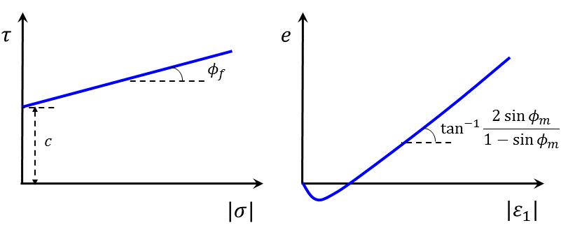
Figure 5: Shear stress versus normal stress (left) and volumetric strain versus axial strain (right).

Initialization of the cap pressure

The cap pressure should be initialized to a value that is consistent with the in-situ stress and takes into account volumetric soil over-consolidation, as applicable. The initial cap pressure is derived from the yield criterion \(f^c\) = 0 (see Equation (7)):

(45)\[p_c = OCR \times \sqrt{{q^2 \over \alpha^2} + p^2}\]

where the over-consolidation ratio, \(OCR\), is an amplification factor larger or equal to 1.

The code automatically assigns an initial value of the evolution parameter, \(e^p\), derived from Equation (24) that is consistent with the initial cap pressure.

Initialization of mobilized friction angle

The mobilized friction angle is an important parameter that should be initialized appropriately to be consistent with the in-situ stresses and accounting for shear over-consolidation, as applicable. The following expression, consistent with Equation (3), can be used to determine the mobilized friction angle for a normally shear-consolidated material:

(46)\[\sin \phi^{nc}_m = {{\sigma_1 - \sigma_3} \over {\sigma_1 + \sigma_3 - 2c \cot \phi_f}}\]

where \(\sigma_1\) and \(\sigma_3\) are the minimum and maximum principal effective stresses in-situ, and \(c\) is the cohesion. Equation (46) follows from the geometrical consideration of Mohr circles presented in Figure 1. The initial state of an over-consolidated soil is prescribed by specifying an initial value of the mobilized friction property that is larger than the normally consolidated value \(\phi^{nc}_m\).

Initialization of friction hardening parameter

By default, the friction hardening parameter \(\gamma^p\) is assumed to be zero under in-situ conditions. Alternatively, the user can choose to exercise the modulus degradation curve starting with a value of \(\gamma^p\) that is larger than zero (see discussion on friction hardening). The following expression can be used to initialize the value of plastic shear strain, consistent with the initial value of mobilized friction, (see Equation (31)):

(47)\[\gamma^p = {{1} \over {\beta(1+R)G_{ref}}} \cdot {{\sin \phi_f \sin \phi_m} \over {\sin \phi_f - \sin \phi_m R_f}}\]

Alternative Features

User-defined hardening/softening laws

One flexible feature of the model is the capability to substitute alternative user-defined hardening/softening laws for the built-in laws, which are communicated to the model by means of tables. Up to five tables can be declared. Tables may specify mobilized friction, dilation, and cohesion in terms of plastic shear strain measure, \(\gamma^p\); tensile strength in terms of tensile plastic strain, \(e^{pt}\); and volumetric cap pressure in terms of cap plastic volumetric strain, \(e^p\). When a table is declared for a specific model property (e.g., friction, dilation, cohesion, tensile strength, or cap-pressure), the associated user-defined law takes precedence over the corresponding built-in law.

Duncan-Chang type model

For geotechnical applications that do not require taking into account substantial plastic volumetric strains, the volumetric cap is usually ignored. On the other hand, it is still important to consider the dependency of the material elastic moduli on the initial effective stresses. This type of problem is often analyzed with the use of the Duncan and Chang hyperbolic soil model (1970).

To account for such behavior in the CYSoil model, the user should specify not to use the volumetric cap by setting flag-cap = 0 (the default value). Also, the user should assign \(p_{ini}\) to a (positive) zone-based measure of initial confinement (e.g., \(p_{ini} = \sigma_3\)). The code will then use the value of \(p_{ini}\) in lieu of \(p_c\) in Equations (19) and (20) for bulk and shear moduli.

The emerging behavior of the model should be similar to that of a Duncan-Chang model (in the case that dilation is fixed at zero, using flag-cap = 1), or that of the CHSoil model in particular.

Constant friction angle

It is possible to use a constant friction angle as an alternative to the built-in friction hardening logic in the CYSoil model. To select this option, the user needs to set flag-shear = 1 (the default is 0) and the input value of the friction property to the desired friction angle.

Dilation alternatives

The built-in dilation logic is used when flag-dilation = 0 (the default value). There are two alternative options: 1) constant dilation (flag-dilation = 1), in which case the input value of the dilation property is used; and 2) Rowe’s Dilation law (flag-dilation = 2), in which case \(\phi_{cv}\) is not internally derived from \(\phi_f\) and \(\psi_f\), but an input value that is set using friction-critical.

Implementation Procedure

The implementation procedure for the CYSoil model follows the general implementation of the double-yield model. At each timestep, new stresses are computed using the current values of the model properties. In this process, an elastic guess, \(\sigma_{ij}^I\), is first computed by adding to the old stress components, increments calculated by application of Hooke’s law to the total strain increment for the step. Principal stresses \(\sigma_1^I, \sigma_2^I, \sigma_3^I\), and corresponding principal directions, are calculated and ordered. If these stresses violate the yield criteria for shear, volume (cap), and/or tension, corrections are applied to the elastic guess to give the new stress state. The stress tensor components in the system of reference axes are then calculated from the principal values by assuming that the principal directions have not been affected by the occurrence of a plastic correction.

The evolution parameters \(\gamma^p\), \(e^p\), and \(e^{pt}\) for shear, cap, and tensile yielding, respectively, are calculated independently by the code. The parameter for shear yielding is the (accumulated) plastic shear strain, \(\gamma^p\); the plastic shear strain increment is defined as

(48)\[ \Delta \gamma^p = \biggl\{\ {1 \over 2} \bigl(\Delta e_1^{ps} - \Delta e^{ps}_m \bigr)^2 + {1 \over 2} \bigl(\Delta e^{ps}_m \bigr)^2 + {1 \over 2} \bigl(\Delta e_3^{ps} - \Delta e^{ps}_m \bigr)^2 \ \biggl\}^{1 \over 2}\]

where \(\Delta e_m^{ps} = \bigl(\Delta e^{ps}_1 + \Delta e^{ps}_3)/3\) and \(\Delta e_j^{ps}, j\) = 1,3 are the principal plastic shear strain increments.

The evolution parameter for cap yielding is the modulus of plastic volumetric strain, \(e^p\), and its increment is defined as

(49)\[ \Delta e^{p} = \vert \Delta e^{p}_1 + \Delta e^{p}_2 + \Delta e^{p}_3 \vert\]

where \(\Delta e_j^{p}, j\) = 1,3 are the principal plastic strain increments from yielding on the cap.

The tensile hardening parameter \(e^{pt}\) measures the accumulated tensile plastic strain; its increment is defined as

(50)\[ \Delta e^{pt} = e_3^{pt}\]

where \(\Delta e_3^{pt}\) is the increment of tensile plastic strain in the direction of the major principal stress (recall that tensile stresses are positive).

The components of the plastic strain increment for each failure mode are evaluated from expressions similar to those derived for the double-yield model. Zone hardening increments are then calculated from the relevant (surface averaged) plastic strain increments for all triangles involved in the zone. After this, new zone properties (e.g., mobilized friction, cohesion, dilation, updated cap pressure) are calculated and stored for use in the next step.

The hardening or softening lags one timestep behind the corresponding plastic deformation. In an explicit code, this error is small because the steps are small. Several simple tests are presented below to illustrate the CYSoil model features and capabilities.

References

Boukpeti, N. Modeling Static Liquefaction in Granular Deposits. Ph.D. Thesis, University of Minnesota (2001).

Byrne, P. M., S. S. Park and M. Beaty. “Seismic Liquefaction: Centrifuge and Numerical Modeling,” in FLAC and Numerical Modeling in Geomechanics — 2003 (Proceedings of the 3rd International FLAC Symposium, Sudbury, Ontario, Canada, October 2003), pp. 321-331. R. Brummer et al., eds. Lisse: A. A. Balkema (2003).

Duncan, J. M., and C. Y. Chang. “Nonlinear Analysis of Stress and Strain in Soils,” Soil Mechanics, 96 (SM5), 1629-1653 (1970).

Rowe, P. W. “The Stress-Dilatancy Relation for Static Equilibrium of an Assembly of Particles in Contact,” Proc. Roy. Soc. A., 269, 500-527 (1962).

cap-yield Model Properties

Use the following keywords with the zone property command to set these properties of the cap-yield (CYSoil) model.

cap-yield

cohesion f

ultimate cohesion, \(c\). The default is 0.0.

dilation f

ultimate dilation angle, \(\psi_f\). The default is 0.0.

friction f

ultimate friction angle, \(\phi_f\). If the specified value is less than 0.1 degree, it will be limited to 0.1 degree for numerical stability.

friction-mobilized f

mobilized friction angle, \(\phi_m\), which should be initialized no less than the value determined by \(\phi^{nc}_m\) (see this equation) via a command or FISH function.

pressure-cap f

cap pressure, \(p_c\), which can be initialized via a command or a FISH function.

pressure-initial f

initial mean effective stress, \(p_{ini}\). Required if pressure-cap is not specified. It can be initialized via a command or a FISH function.

pressure-reference f

reference pressure, \(p_{ref}\). A non-zero value should be specified based on the unit of stress/pressure adopted in the model.

poisson f

current Poisson’s ratio, \(\nu\). The default is 0.2.

shear-reference f

dimensionless elastic shear modulus reference value, \(G_{ref}\). A non-zero value should be specified.

tension f

tension limit, \(\sigma^t\). The default is 0.0.

alpha f (a)

dimensionless cap yielding surface parameter, \(\alpha\). The default is 1.0.

beta f (a)

dimensionless calibration factor, \(\beta\). The default is 1.0.

dilation-mobilized f (a)

current mobilized dilation angle, \(\psi_m\). It is read-only, except for table-dilation ǂ 0.

exponent f (a)

exponent for the pressure-dependent elastic moduli, \(m\). The default is 0.5, and the upper limit is 0.99.

failure-ratio f (a)

failure ratio, \(R_f\). The default is 0.9.

flag-brittle b (a)

If true, the tension limit is set to 0 in the event of tensile failure. The default is false.

flag-cap i (a)

= 0 (default), no cap. The elastic moduli are functions of the mean effective stress, and pressure_initial should be specified.

= 1, with cap. The elastic moduli are functions of the cap pressure and pressure_cap should be specified via a command or a FISH function, or calculated internally otherwise, see information on pressure_cap.

flag-dilation i (a)

= 0 (default), the built-in Rowe dilation rule is used.

= 1, \(\psi_m\) ≡ \(\psi_f\).

= 2, \(\phi_{cv}\) should be specified and \(\psi_m\) is calculated from this equation.

flag-shear i (a)

= 0 (default), the built-in shear hardening law is used.

= 1, \(\phi_m\) ≡ \(\phi_f\).

friction-0 f (a)

initial mobilized friction angle, \(\phi_0\) associated with zero plastic shear strain. By default, \(\phi_0\) = \(\phi_m\) if \(\epsilon_{ps}\) is initialized to 0.0; otherwise, \(\phi_0\) = 0.0 if not specified.

friction-critical f (a)

constant \(\phi_{cv}\). The default value is calculated by this equation. Required for specification only if flag-dilation = 2.

over-consolidation-ratio f (a)

over-consolidation ratio, \(OCR\). The default is 1.0.

multiplier f (a)

multiplier on current plastic cap modulus to give elastic bulk and shear moduli, \(R\). The default is 5.0 with cap and 0.0 without cap.

shear-maximum f (a)

maximum (upper-bound limit) of the elastic shear modulus, \(G^e_{max}\). The default internally calculated value is \(10 \times G^e_{ini}\), where \(G^e_{ini}\) is the initial \(G^e\) when the model is first time set up.

shear-minimum f (a)

minimum (lower-bound limit) of the elastic shear modulus, \(G^e_{min}\). The default internally calculated value is \(0.1 \times G^e_{ini}\), where \(G^e_{ini}\) is the initial \(G^e\) when the model is first time set up.

strain-shear-plastic f (a)

accumulated plastic shear strain, \(\gamma^p\). By default, it is initialized internally.

strain-tensile-plastic f (a)

accumulated plastic shear strain, \(e^{pt}\). The default initial value is 0.0.

strain-volumetric-plastic f (a)

accumulated plastic volumetric strain, \(e^p\). By default, it is initialized internally.

table-pressure-cap s (a)

name of the table relating cap pressure to plastic volume strain.

table-cohesion s (a)

name of the table relating cohesion to plastic shear strain.

table-dilation s (a)

name of the table relating mobilized dilation angle to plastic shear strain.

table-friction s (a)

name of the table relating mobilized friction angle to plastic shear strain.

table-tension s (a)

name of the table relating tensile strength to plastic tensile strain.

void-initial f (a)

initial void ratio, \(\hat{e}_{ini}\). The default is 1.0.

void-maximum f (a)

allowable maximum void ratio, \(\hat{e}_{max}\). The default is 999.0, a virtual value to bypass the dilatancy cut-off.

bulk f (r)

current elastic bulk modulus

pressure-effective-cy f (r)

mean effective stress, \(p\)

shear f (r)

current elastic shear modulus

stress-deviatoric-cy f (r)

deviatoric stress, \(q\)

void f (r)

current void ratio, \(\hat{e}\)

young f (r)

current elastic Young’s modulus, \(E\)

Key

(a) Advanced property.

This property has a default value; simpler applications of the model do not need to provide a value for it.

(r) Read-only property.

This property cannot be set by the user. Instead, it can be listed, plotted, or accessed through FISH.

Notes

• The tension cut-off is \({\sigma}^t = min({\sigma}^t, c/\tan \phi)\).

• One parameter between \(p_c\) and \(p_{ini}\) must be specified.

• The void related parameters, \(\hat{e}_{ini}\) and \(\hat{e}_{max}\), are for dilatancy cut-off only. If dilatancy cut-off is not taken into account, these parameters are not required for input (default values are used).

• The tension table and flag-brittle should not be active at the same time.