Elastic Beam with Concentrated Loads (with shell elements)
Problem Statement
Note
To view this project in FLAC3D, use the menu command . The data file used is shown at the end of this example.
The maximum midspan deflection, shear-force, and bending-moment distributions for a long thin beam simply supported and loaded by two concentrated loads are computed and compared with the analytical solution for an Euler-Bernoulli beam. The problem is modeled with Euler-Bernoulli beam elements in Elastic Beam with Concentrated Loads. The problem is here modeled with DKT plate-bending elements. This problem describes how a plate manifests greater stiffness than a beam, and quantifies the ability of the DKT plate-bending element to model the bending action.
Analytical Solution
The analytical solution is given in Elastic Beam with Concentrated Loads. The solution corresponds with simple beam theory assumptions. Ugural (1981, p. 8) describes how these assumptions differ for plate theory:
\(\ldots\) if a plate element of unit width and parallel to the beam axis were free to move sidewise under transverse loading, the top and bottom surfaces would be deformed into saddle-shaped or anticlastic surfaces \(\ldots\) The flexural rigidity would then be \(E t^3 / 12\), as in the case of a beam. The remainder of the plate prevents the anticlastic curvature however. Owing to this action, a plate manifests greater stiffness than a beam by a factor \(1 / (1 - \nu^2) \ldots\)
For the present problem, we need to set Poisson’s ratio of the plate equal to zero in order to match the solution from simple beam theory.[1]
Particular Problem
The particular problem to be considered is defined as follows. The plate has a 9-m length, 1-m depth and 100-mm thickness. The plate is comprised of structural steel, and is assumed to behave as an isotropic elastic material with
The Young’s modulus of the plate is set to \(E\), and the Poisson’s ratio of the plate is set to zero (for the reason cited above). Each concentrated load \((P = 1 \times 10^4 \textrm{ N})\) is applied as a constant force-per-unit-length \((P / b)\) that acts over the plate depth. For these properties, the maximum midspan deflection is given by the simple beam theory solution of \(15.5312 \textrm{ mm}\).
FLAC3D Model
The beam is modeled as a finite-sized rectangular plate of length \((L)\), width \((b)\) and thickness \((d)\) using a 9 by 3 mesh of DKT elements with a cross-diagonal pattern as shown in Figure 2. The cross-diagonal pattern is used to ensure symmetric response. The simply-supported boundary condition (translational velocity fixed in the \(y\) direction) is assigned to the nodes along the \(x = 0\) and \(x = L\) lines. The concentrated loads are applied as constant forces-per-unit-length along the \(x = 3\) and \(x = 6\) lines. The \(y\)-displacement at the plate center is monitored as a history. Local nonviscous damping is used with a damping factor of 0.8. The model is run in small-strain mode to correspond with the small-strain assumption of the analytical solution. The model is cycled until a convergence limit of \(1 \times 10^{-3}\) is achieved.
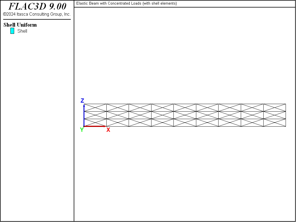
Figure 1: Geometry of the FLAC3D model showing mesh and global coordinate system.
Results and Discussion
The deformed shape and center-deflection history are shown in Figure 2, from which we conclude that the static solution has been obtained. The maximum deflection occurs at the center and equals \(15.5216 \textrm{ mm}\), which is within 0.06% of the analytical solution. The displacement field in Figure 3 is visualized using the plot item, checking the box, and assigning a deformation factor of 50. The displacement field can also be visualized as displacement vectors (arrows) that emanate from each node via the plot item as shown in Figure 3.
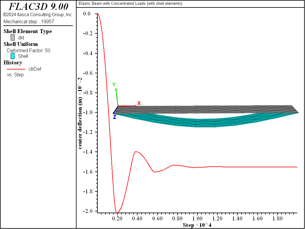
Figure 2: Deformed shape (deformation factor: 50), undeformed shape and center deflection.
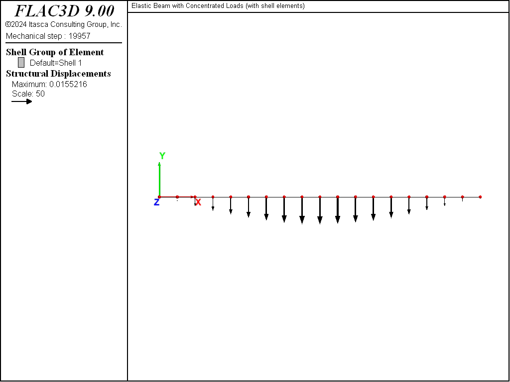
Figure 3: Displacement field plotted as displacement vectors on undeformed shape.
The stress resultants are expressed in terms of the surface coordinate system shown in Figure 4. The bending moment is equal to the \(M_x\) stress resultant multiplied by the plate depth (of unity), and the shear force is equal to the \(Q_x\) stress resultant multiplied by the plate depth (of unity). The stress resultant field variations are displayed as contours using the plot item, setting the surface-X vector () equal to \((1,0,0)\), and unchecking the box (discussed here).
The shear-force and bending-moment distributions are shown in Figures 5 and 6. The shear-force distribution corresponds exactly with the analytical solution. The bending-moment distribution matches the analytical solution except at the plate ends. The values at the ends are not zero, but will approach zero as the mesh is refined.
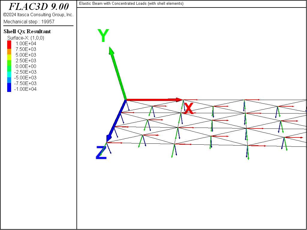
Figure 4: Surface coordinate system ({red, green, blue} = {x, y, z}) and global coordinate system (large arrows).
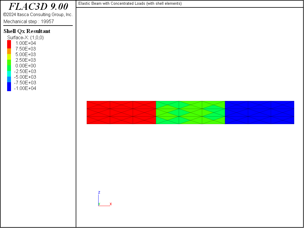
Figure 5: Shear-force distribution.
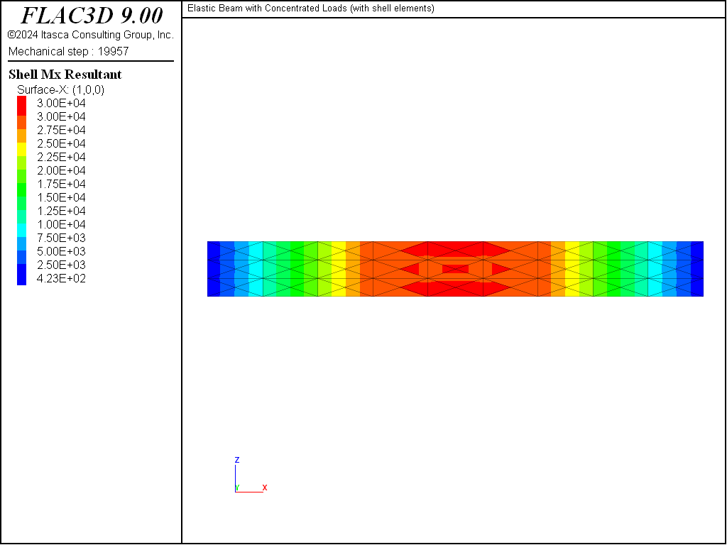
Figure 6: Bending-moment distribution.
Reference
Ugural, A. C. Stresses in Plates and Shells. New York: McGraw-Hill Publishing Company Inc. (1981).
Endnotes
Data File
ConcentratedLoadsShell.dat
model new
model title 'Elastic Beam with Concentrated Loads (with shell elements)'

; Create shell elements and assign material properties.
structure shell create by-quadrilateral (0,0,0) (9,0,0) (9,0,1) (0,0,1) ...
                    size=(9,3) cross-diagonal element-type dkt
structure shell property thickness 0.1
structure shell cmodel assign elastic
structure shell property young 200e9 poisson 0.0

; Specify boundary conditions (including applied loads).
structure node fix velocity-y range position-x 0.0 position-x 9.0 union
structure node apply force-edge (0,-1e4,0) range position-x 3.0 position-x 6.0 union

; Setup history for monitoring behavior.
structure node history name 'ctrDef' displacement-y position (4.5, 0, 0.5)  ; plate center

model large-strain off
structure mechanical damping local 0.8
model solve convergence 1e-3
model save 'ConcentratedLoadsShell'
| Was this helpful? ... | Itasca Software © 2024, Itasca | Updated: Nov 12, 2025 |
