Examples • Example Applications
Slope Stability for a Cohesive and Frictional Soil (FLAC2D)
Problem Statement
Note
This project reproduces Example 1 from FLAC 8.1. The project file for this example is available to be viewed/run in FLAC2D.[1] The project’s main data files are shown at the end of this example.
A common problem encountered in engineering soil mechanics is the stability of soil slopes in frictional materials. In this example, three slope conditions are analyzed. First, a slope in sand with zero cohesion is modeled with an initial slope steeper than the angle of repose of the sand. This slope, of course, should collapse; the progression of this collapse is calculated as it develops. Second, a small cohesion is added to the material and the slope is reexamined to determine whether it is stable. Third, the water level in the slope is raised, and the effect on stability is examined.
In this example, the soil is homogeneous, and the stability and factor of safety of the slope can readily be determined using an analytic or graphical technique. However, the power of the FLAC2D code is in its ability to model more complex slope geometries in which, for example, several layers of soil with differing material properties and/or constitutive behaviors may exist. This type of problem can be examined with no greater effort than needed for the homogeneous case by simply assigning different material properties and/or models to different zones.
This example also demonstrates two approaches to analyze the effect of a phreatic surface in the slope. In one approach, an effective-stress analysis is performed after adding a pore-pressure distribution directly to the zones in the model. In the other approach, a groundwater flow calculation is performed first to establish the phreatic surface; then the effective-stress analysis is performed.
Modeling Procedure
Model Geometry
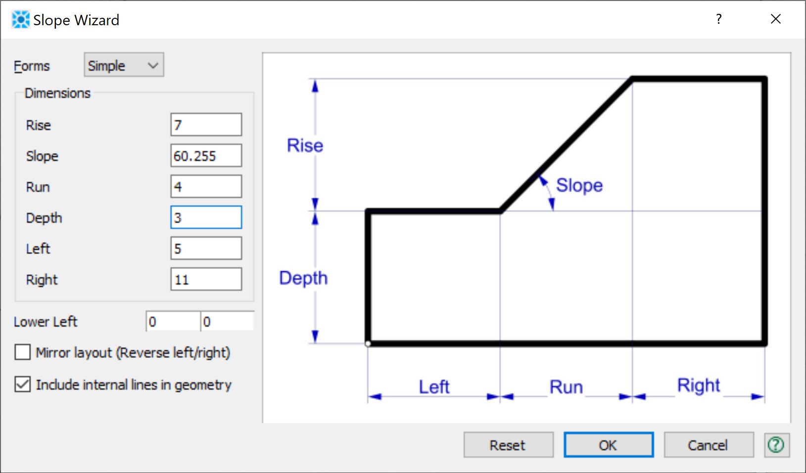
The model zones are created in a sketch using the Slope Wizard tool. After opening the slope wizard, fill in the form as shown. Note that slope angle is automatically calculated in the dialog based on the other dimensions.
The model simulates ponded water on the left side at a height of 5 m. To make it easier to apply the necessary boundary conditions, it is useful to have a point on the slope at y = 5. Use the line tool (![]() ) from the “Point/Edge Tools” dropdown to put a horizontal line at y=5 that extends from beyond the the left of the slope to the right side of the model. The intersection point on the slope face will be automatically calculated. Then delete the dangling line segment to the left of the slope face by clicking on the extraneous point and deleting it.
) from the “Point/Edge Tools” dropdown to put a horizontal line at y=5 that extends from beyond the the left of the slope to the right side of the model. The intersection point on the slope face will be automatically calculated. Then delete the dangling line segment to the left of the slope face by clicking on the extraneous point and deleting it.
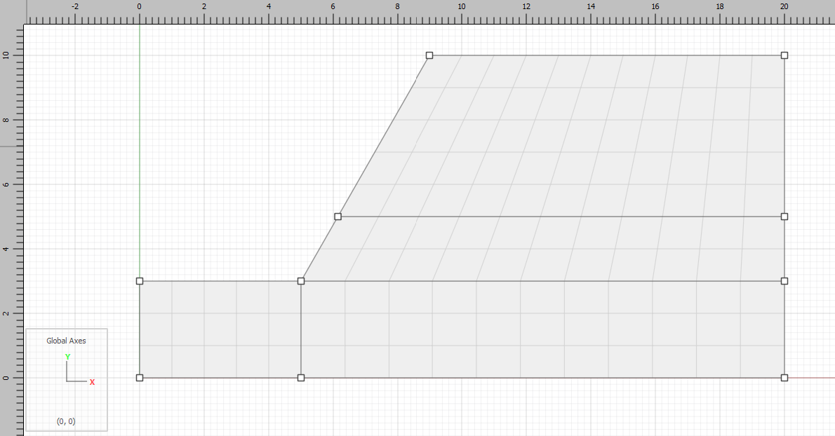
Next use autosize (![]() ) on the “Mesh Tools” pulldown to set zone length to 1. Then use mesh all polygons (
) on the “Mesh Tools” pulldown to set zone length to 1. Then use mesh all polygons (![]() ), also on the “Mesh Tools” pulldown, to add zones to the model blocks. The model should appear as shown:
), also on the “Mesh Tools” pulldown, to add zones to the model blocks. The model should appear as shown:
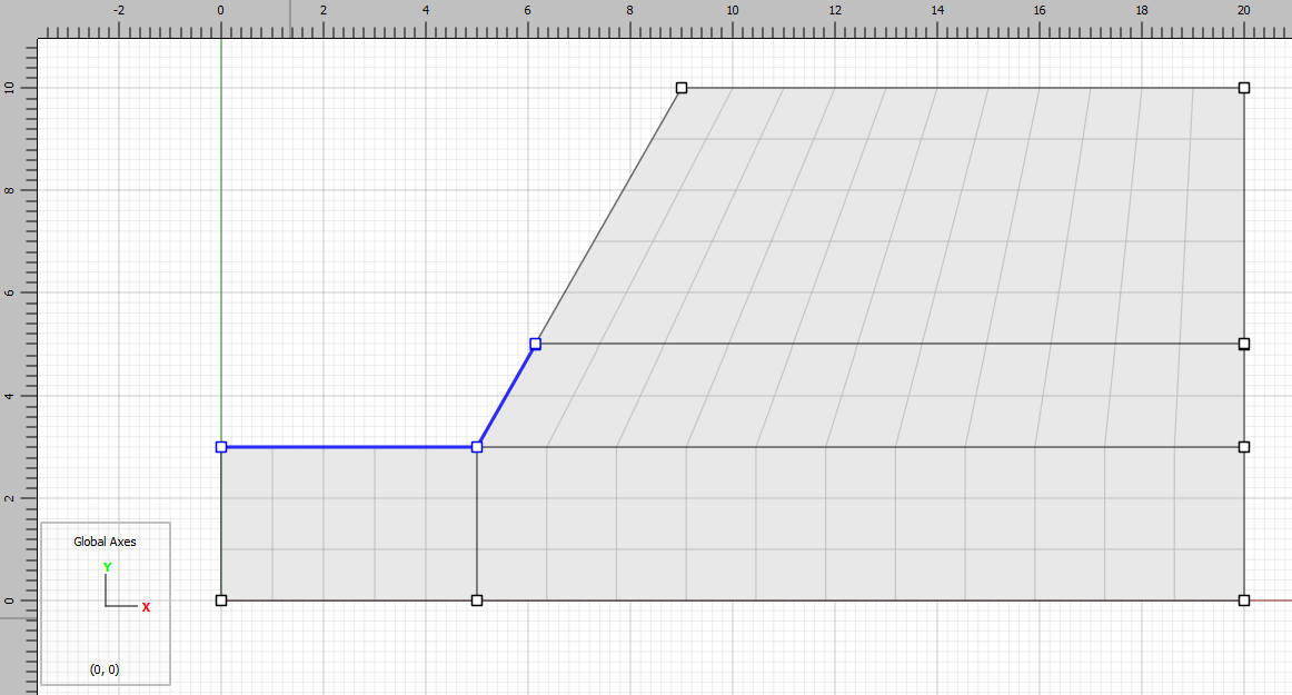
Finally, select the segments of the slope that will be under water, access their “group” property, and assign them a group name of water_surface.
Press the create zones button (![]() ) to create the zones.
) to create the zones.
Model Properties
From the Model view in the workspace, select all of the zones (ctrl-A), select assign a constituive model… ( ) from the “Commands” pulldown and assign the Mohr-Coulomb constitutive model. Then, with all zones still selected, select set model properties … (
 ) from the same pulldown to assign properties as shown below:
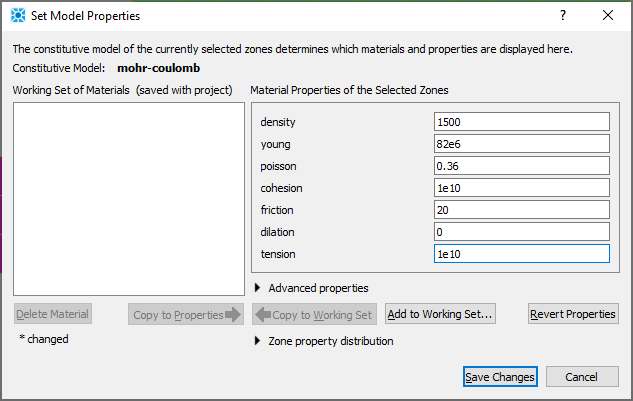
Pa stress units are used for this example. Note that a high cohesion and tensile strength are assigned to prevent slope failure during the initialization of gravitational stresses in the model.
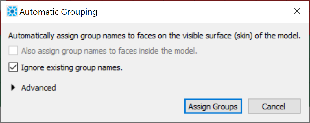
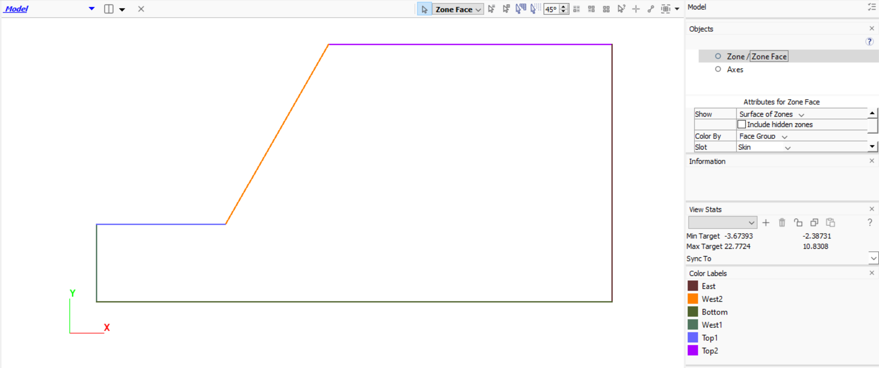
Now, group names are assigned to the faces to facilitate indentifying them later when applying boundary conditions. Click the Assign group names to faces automatically … button (![]() ) on the toolbar. Uncheck the first box and check the second box as shown:
) on the toolbar. Uncheck the first box and check the second box as shown:
In the Model view, make sure Skin is selected for the “Show” attribute in the “Attributes for Zone Face” list to the right of the plot. The face groups should appear as shown below.
Save the project and the model state. It is also a good idea to go to the tab in the Commands area and press the Save to File as Data File… button (![]() ). This creates a data file that preserves all the commands that have been issued interactively up to this point.
). This creates a data file that preserves all the commands that have been issued interactively up to this point.
Initial Model State
The commands required to bring the model to initial equilibrium state are shown in the data file initial.dat.
The boundary conditions consist of roller boundaries on the left and right sides of the model, as well as a fixed base. The acceleration of gravity is set to 9.81 m/sec2 (positive means acting downward). An initial elastic state in which gravitational stresses are equilibrated is desired. This is achieved with the model solve command, using default limits. Equilibrium is obtained when the out-of-balance force ratio limit of 10:sup`-5` is reached. To examine the progression of the solution, the \(y\)-displacement history is requested at a gridpoint at the slope crest. This is done using the zone history command. When the model solve command has reached its limit, the history may be plotted to verify that the mesh is indeed at an equilibrium state.
Initially, very large values for the cohesion and tensile strength are assigned to the slope. This can be justified by reexamining the way an explicit model works. An initial grid is created first and, in this case, gravity is applied to the gridpoints. Gravitational stresses are allowed to equilibrate. For most problems, it is desirable that this process occur as rapidly as possible. This can be done by requiring the material to behave elastically during the equilibration process.
Once stresses have equilibrated, actual material properties are assigned, excavation occurs, loads are applied, etc., and the simulation process continues. In the case illustrated here, a plastic constitutive model is assigned initially, with high cohesion and tensile strength, forcing the material to behave elastically. Then the cohesion and tensile strength are reset to the desired values. Note that the same result could be achieved by using the command model solve elastic only, or by assigning an elastic constitutive model to the zones for this step.
A save file is created to save the elastic equilibrium state using the command model save. This is done to save time in case future runs will be made in which material parameters or constitutive models are varied. Performing these studies requires only that the elastic state be restored, therefore eliminating the necessity of recomputing the equilibrium state. In the next step, this state will be restored with the model restore command.
Slope Collapse: Dry Conditions
For the next stage of the simulation, the material properties are set to the actual soil values and the calculation is continued while examining the possible failure process. During this process, plots of the progressive displacement of the slope are made. To avoid any confusion in analyzing the data, only the change in displacement is monitored, not the cumulative displacements from the beginning of the simulation. The calculation procedure in FLAC2D does not involve displacements, but keeps the cumulative total for each gridpoint as a convenience to the user. Therefore, the displacements may be initialized at any point in the run without affecting the results. This is done by using the command zone gridpoint initialize displacement and setting the \(x\) and \(y\) displacements to 0.
From this point on, plots will show only the change in displacement from the previous state.
Next, the material properties of the zones are reset by using the zone property command. The cohesion is set to zero for all zones (note that the tension strength is automatically set to 0 since the maximum tension strength equals cohesion/tan(friction). Finally, the calculation mode is set to large-strain to provide a more accurate geometrical representation of the slope failure as it progresses. Because slope collapse will occur due to the angle of repose of the soil being smaller than the slope angle, the model solve command is not used——equilibrium will not be reached. The model cycle command is used to proceed the simulation in small increments of calculational steps, stopping at each increment to print and plot intermediate stages. Here, the power of the explicit method is evident in its ability to follow highly nonlinear problems—which may never converge to an equilibrium state—through progressive failure.
The model is now stepped in intervals to evaluate the progressive collapse of the slope. The collapse is revealed when printing and plotting results after each model cycle.
Figures 7 and 8 show the state of the slope after 100 steps and after an additional 500 steps. These figures illustrate the progressive collapse and, in particular, indicate the location of the failure (slip) surface. The slope is collapsing in an attempt to reach its angle of repose. At some point, the displacements of the gridpoints become unrealistic because of extreme distortion of the grid. FLAC2D automatically checks for excessive grid deformation and will stop the calculation process if the condition is detected, displaying an error message.
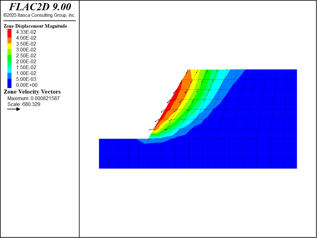
Figure 7: Velocity contours and displacement vectors after running 100 steps at 0 cohesion. Note that the scale for the vectors was set to 0.1 (10% of the model size), rather than the default 0.05 to make the vectors larger.
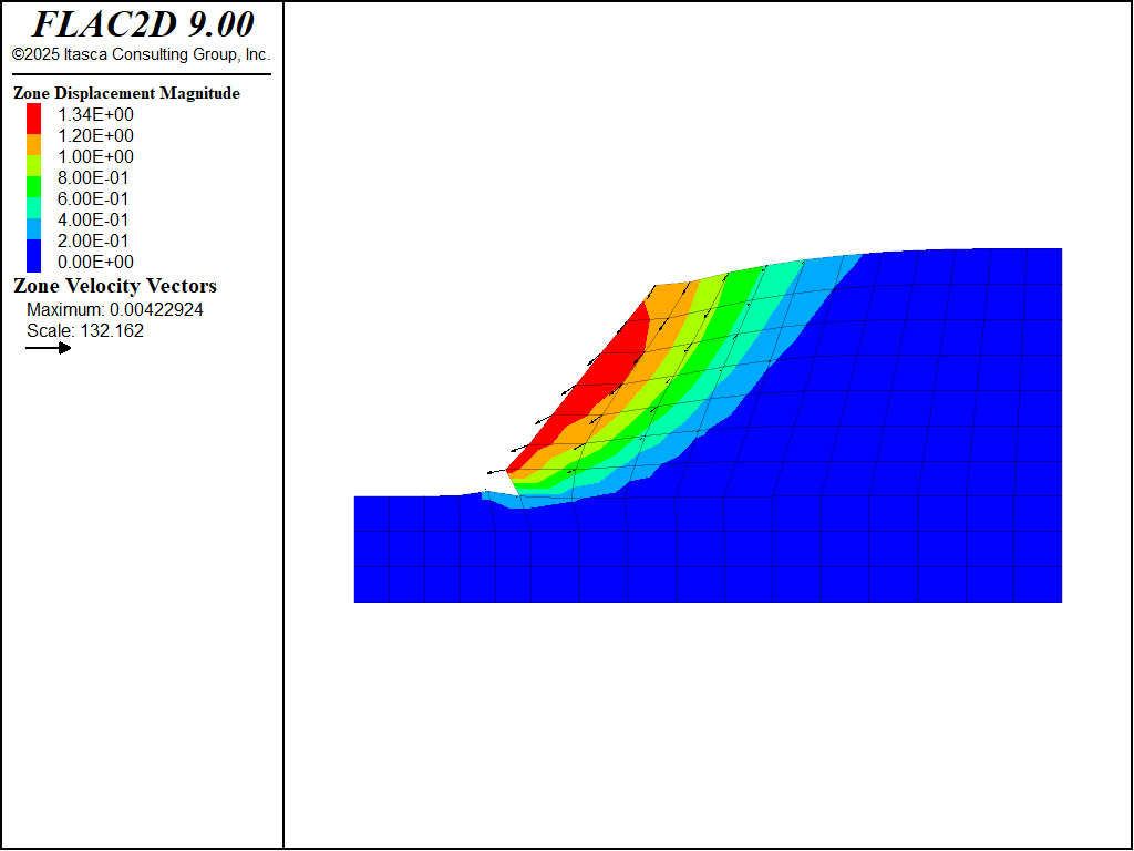
Figure 8: Velocity contours and displacement vectors after running 600 steps at 0 cohesion.
An interesting comparison can be obtained by running another simulation in which a small cohesion and zero tensile strength are assigned to the soil. Because the initial elastic equilibrium state has been saved, the problem can be restored from this state. The displacements are then reset, the properties are changed and the model is solved.
model restore 'initial'

zone gridpoint initialize displacement 0 0

zone property cohesion 1e4 tension 0

model solve
Under these conditions, the results will show that the slope is stable. (Note the small magnitude of the calculated displacements in Figure 9.)
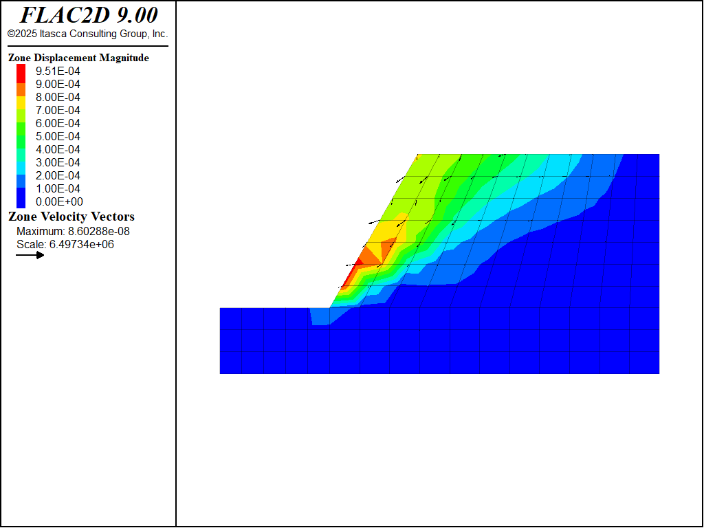
Figure 9: Velocity contours and displacement vectors after solving with cohesion = 10 kPa.
Effective Stress Analysis with water table
Next, the stability of the slope with a water table present is assessed. Continuing with the model at the present state, the water level is raised in the slope to a height of 9 m on the right side of the model and 5 m on the left side (i.e., 2 m above the base of the excavation).
For a planar water table, simply use the zone water command with the plane keyword and give the plane location and orientation. For a non-planar water table, the water table must first be defined as a geometry. This can be done with commands as shown below.
geometry set 'water_table'
geometry edge create by-positions (0,5) (6.11,5) (20,9)
The name assigned to the geometry set is not important. The geometry set is then specified when giving the water table command and pore-pressures will be automatically calculated (assuming the water density has been specified first). CS: this entire paragraph is wonky. There is no water table command, and the statement about the name’s importance is unclear.
Note that the correct wet and dry densities must also be supplied. The zones below the geometry surface can be identified using a range: range geometry-space 'water_table'. Giving the qualifier count 1 to this range specifies that any zone that is below the water table will be identified (a ray is cast upwards from each zone centroid, and if the ray intersects the geometry surface 1 times, the zone will be selected). Assuming a porosity of 0.3, the wet density can therefore be assigned as shown.
[wet_dens = 1500 + 1000*0.3]
zone property density [wet_dens] ...
  range geometry-space 'water_table' count 1
The square brackets [ ] denote inline FISH that can be used to make simple calculations or refer to FISH variables inside of commands.
The zone face apply command must also be used to apply the weight of the water in the excavation to the surface of the excavation. This is where previously setting the face groups in the sketch set comes in handy. The required command is:
zone face apply stress-normal [-5*1000*9.81] gradient 0 [1000*9.81] ...
  range group 'water_surface'
For both pore pressure and stress boundary conditions, the value given is the value at (0,0) and the gradient is the change per unit length in the vertical (positive z) direction.
Note
The equivalent example in FLAC 8.1 incorrectly states that this model fails. In fact, it also reaches equilibrium with a SOLVE command and shows similar displacements.
Figure 10 illustrates the location of the water table, the applied forces representing the weight of the water in the excavation, and the wet and dry densities in the zones.
The calculation is continued with the model solve command. The model reaches equilibrium, but the displacements are much larger than in the model with no water. (Figure 11).
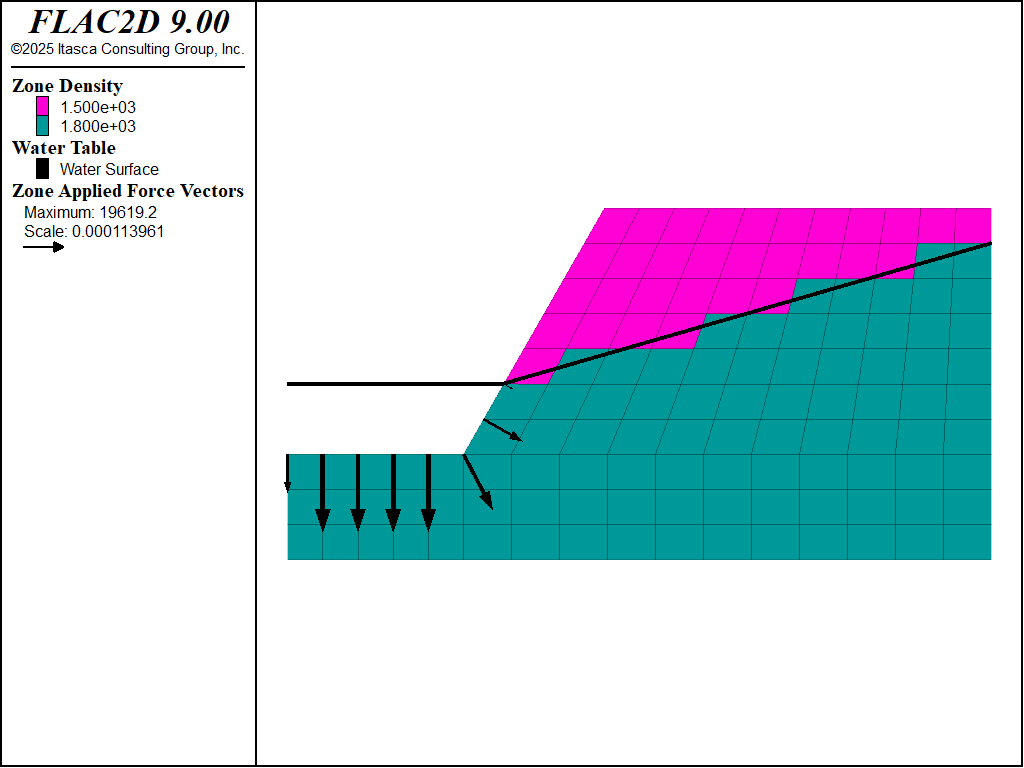
Figure 10: Location of water table, applied forces along slope, and wet and dry densities.
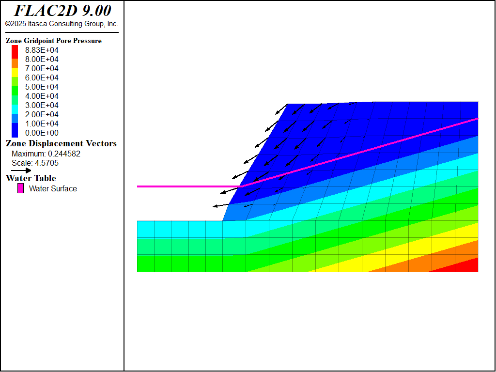
Figure 11: Pore-pressure contours and displacement vectors after solving with cohesion = 10 kPa.
Effective Stress Analysis with water flow
Alternatively, the groundwater flow capabilities in FLAC2D can be used to find the phreatic surface and establish the pore pressure distribution before the mechanical response is investigated. The model is run in groundwater flow mode by using the model config fluid command.
To perform the fluid flow analysis, the mechanical calculation is turned off (model mechanical off) in order to establish the initial pore pressure distribution. Pore pressure boundary conditions are applied to raise the water level to 5 m at the left boundary and 9 m at the right. By default, when fluid model is turned on, the slope is assumed to be wet (initial saturation 1). The zones then desaturate as the calculation progresses. You could do the reverse by setting all of the saturation to 0 and allowing it to become wet. The steady-state result will be the same.
Also, the bulk modulus of the water is set to a low value (1.0 × 10⁴) because the objective is to reach the steady-flow state as quickly as possible. The groundwater time scale is wrong in this case, but transient time response is not of interest. The steady-flow state is determined by using the model solve command and specifying a solve condition for the fluid. When the groundwater flow ratio falls below the set value of 0.001, steady-state flow is achieved. The steady-flow state is indicated by the plot of flow vectors and phreatic-surface contour in Figure 12 (when the model is configured for fluid flow, the water table is plotted where saturation = 0.5). The bumpy phreatic-surface line is due to the coarse discretization.
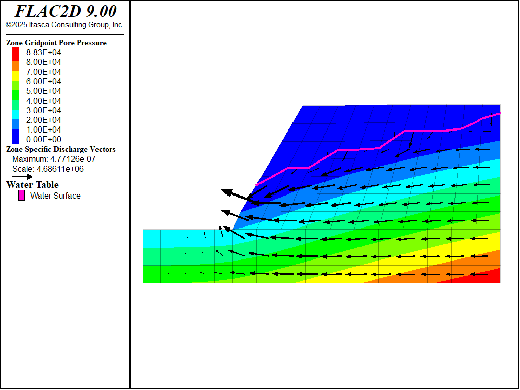
Figure 12: Steady-state flow through the slope.
Mechanical equilibrium is then established including the effect of the previously calculated pore pressure. This is accomplished with the commands
model mechanical active on
model fluid active off
zone gridpoint initialize fluid-modulus 0
These commands turn off the flow calculation, turn on the mechanical calculation, and set the bulk modulus of the water to zero. The last command prevents pore pressures from generating as a result of mechanical deformation. This is done so that the results can be compared to the previous case using the water table. The model cycle command is then used to calculate the mechanical response. Note that the calculated water table is slightly higher than the table specified manually above, so the model is not stable. (Figure 13).
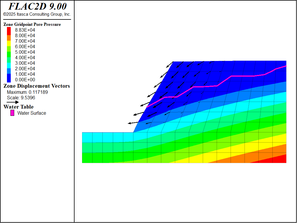
Figure 13: Pore-pressure contours and displacement vectors after 500 steps with cohesion = 10 kPa, using pore pressures calculated from fluid flow analysis.
The approach using the groundwater flow mode can take longer to reach a solution because of the extra calculation needed to establish the pore pressure distribution. However, this method is helpful when the pore pressure distribution or phreatic surface location is unknown. Also, this approach avoids the necessity of assigning wet density values to zones beneath the phreatic surface.
Data Files
initial.dat
model new

; commands produced by sketch and model pane
program call 'model.dat'

zone face apply velocity-x 0 range group 'West1' or 'East'
zone face apply velocity 0 0 range group 'Bottom'

model gravity 9.81

zone history displacement-y position 9,10

model large-strain on
model solve

model save 'initial'
dry-coh0.dat
model restore 'initial'

zone gridpoint initialize displacement 0 0

zone property coh 0

model cycle 100
model cycle 500

model save 'dry-cohesion0'
dry-coh1e4.dat
model restore 'initial'

zone gridpoint initialize displacement 0 0

zone property cohesion 1e4 tension 0

model solve

model save 'dry-cohesion1e4'
water_table.dat
model restore 'dry-cohesion1e4'

zone water density 1000

; make geometry set to define plane
geometry set 'water_table'
geometry edge create by-positions (0,5) (6.11,5) (20,9)

; set water table. Pore pressures will be calculated
zone water set 'water_table'

; set wet density for zones below the water table
; assume a porosity of 0.3
[wet_dens = 1500 + 1000*0.3]
zone property density [wet_dens] ...
  range geometry-space 'water_table' count 1

; apply stress to account for the weight of the ponded water
zone face apply stress-normal [-5*1000*9.81] gradient 0 [1000*9.81] ...
  range group 'water_surface'

model solve

model save 'water_table'
fluid_flow.dat
model restore 'dry-cohesion1e4'

model configure fluid
zone fluid cmodel assign isotropic
zone fluid property permeability 1e-10 porosity 0.3

zone water density 1000

zone gridpoint initialize fluid-modulus 10000
zone gridpoint initialize fluid-tension 0

; water table at 9 m on the right
zone gridpoint fix pore-pressure [1000*9.81*9] gradient 0 [-1000*9.81] ...
  range position-x 20

; water table at 5 m on the left
zone gridpoint fix pore-pressure [1000*9.81*5] gradient 0 [-1000*9.81] ...
  range group 'water_surface'

; apply stress to account for the weight of the ponded water
zone face apply stress-normal [-1000*9.81*5] gradient 0 [1000*9.81] ...
  range group 'water_surface'

; take history and solve fluid
zone history pore-pressure position 10 3
model mechanical active off
model solve fluid ratio-flow 1e-3
model save "fluid_flow_1"

===================

; solve for solid
model mechanical active on
model fluid active off
zone gridpoint initialize fluid-modulus 0

model cycle 500
model save "fluid_flow_2"
Endnote
⇐ Simulation of Pull-Tests for Fully Bonded Rock Reinforcement (FLAC2D) | Axisymmetric Modeling of Post-Pillar Mining (FLAC2D) ⇒
| Was this helpful? ... | Itasca Software © 2024, Itasca | Updated: Nov 12, 2025 |
