Examples • Example Applications

Axisymmetric Modeling of Post-Pillar Mining (FLAC2D)

Problem Statement

Note

This project reproduces Example 2 from FLAC 8.1. The project file for this example is available to be viewed/run in FLAC2D.[1] The project’s main data files are shown at the end of this example.

Post pillars are created when mechanized cut-and-fill stopes are mined on all sides, creating a long thin pillar that is confined by backfill. This example is an examination of the potential instability of a post pillar.

The axisymmetric geometry in FLAC2D is used to approximate the post-pillar mining state. The axisymmetry provides an analysis of pillar deformation closely related to the three-dimensional condition (FLAC3D is recommended for a more rigorous three-dimensional analysis).

Modeling Procedure

Model Geometry

Note

The model geometry is a bit different than the equivalent model in the FLAC 8.1 documentation. The present example uses higher-resolution zoning and the places boundaries further from the excavations to give more accurate results.

The post-pillar is modeled as a cylinder with a radius of 10 m. The width of the stope is 20 m. The model is constructed in a sketch set. First, a rectangle with dimensions of 150 x 160 is created. Note that for an axisymmetric model, the left edge must lie on the \(y\)-axis (\(x\)=0). Five excavations are then created by drawing horizontal lines \(y\)=50, 60, 70, 80, 90 and 100. Vertical lines are then drawn at \(x\)=10 and \(x\)=30.

The model is zoned by selecting Auto-size… (), specifying 2.5 for “zone length”, then selecting Mesh All Polygons ().

The model can be made more efficient by grading the zone size away from the region of interest. Access the Object Properties in the Tools area for each of the following. Select the bottom left vertical boundary (from \(y\)=0 to \(y\)=50) and change “Zone number” to 10 set “Ratio” to 1.1. Repeat for the top left vertical boundary. Now click on the top right boundary (from \(x\)=30 to \(x\)=16) and change “Zone number” to 20 and set “Ratio” to 1.1. Figure 1 shows the resulting mesh.

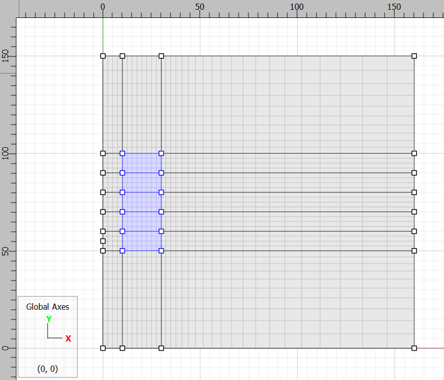
Figure 1: Mesh for pillar model; intended excavation regions are highlighted.

The different excavation stages are assigned group names, ex1 to ex5 from bottom to top. Select each block and set its name by accessing the block’s “Group” property in the “Object Properties.” The zones are then created by clicking the Create Zones () button.

After the zones are created, a new plot is created and zones added to the plot. The zone groups in the Construction slot are shown in Figure 2.

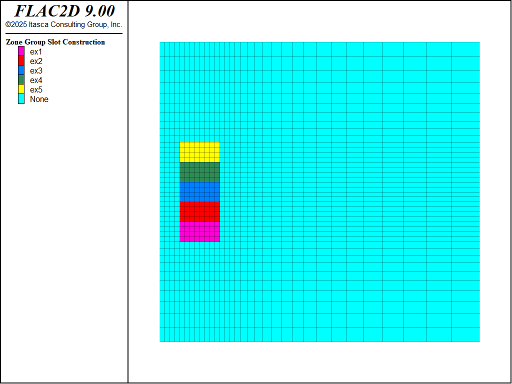
Figure 2: Zone groups.

After zones are created, the commands for constructing the mesh are saved using the State Record tab in the Commands area. The record is exported as a data file () named geometry.dat to allow it to be called later. This is necessary because in an axisymmetric model, the model must be configured for axisymmetry before zones are created (see model config). To do this, first the model is cleared (model new), then configured for axisymmetry, and then the saved data file that stored the sketch commands is called to create the zones.

model new
model configure axisymmetry
program call 'geometry'

Model Staging

Note

The model shown here differs from the same model in the FLAC 8.1 manual in that a small amount of cohesion and tension strength are specified for the backfill. This is necessary since the parameters from FLAC 8.1 produce a situation that is on the verge of instability, so very small differences in model geometry, or solve criteria, can cause large differences in the observed response.

The rock is assigned Mohr-Coulomb material. Properties are as shown in the data file. The constitutive model and properties can be assigned through the Model view in the Workspace, or with commands. Each excavation stage is then excavated by setting the constitutive model to null, and solving. The excavation is then backfilled. Two different scenarios are presented: the first with a Mohr-Coulomb backfill material, and the second with a Double-Yield material. The shear strength properties are the same for both models (friction angle = 35 degrees; cohesion = 0). For the double-yield model, the cap pressure varies from 0.01 MPa at zero plastic volumetric strain, to 50 MPa at a plastic volumetric strain of 0.2.

After backfilling, the next excavation is performed, and so on.

In this model, stress boundary conditions are applied to the top, bottom and right boundary. It is not necessary to specify boundary conditions to the left boundary since this is the center of rotation for the axisymmetric model.

Results

Figure 3 illustrates the history of horizontal displacement at the midpoint of the wall of the pillar following the first cut. This figure indicates that the wall is stable.

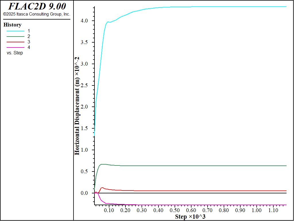
Figure 3: History of horizontal displacement at midpoint of pillar wall following excavation of first cut.

Figures 4 through 8 show the stress trajectories for successive mining stages. As seen, the sandfill does not develop appreciable load, and the pillar becomes de-stressed in the horizontal direction. These plots are from the run with the Mohr-Coulomb model; the results are similar for the run with the double-yield model.

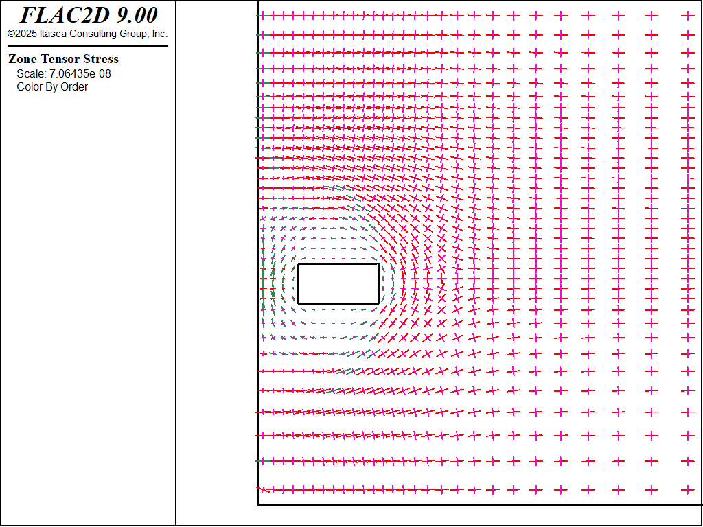
Figure 4: Principal stresses after first cut.

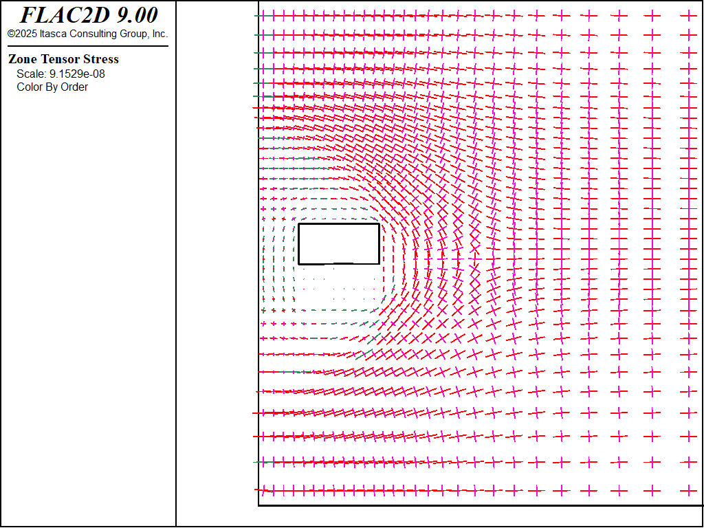
Figure 5: Principal stresses after second cut and fill of first cut (M-C sandfill).

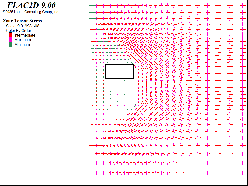
Figure 6: Principal stresses after third cut and fill of second cut (M-C sandfill).

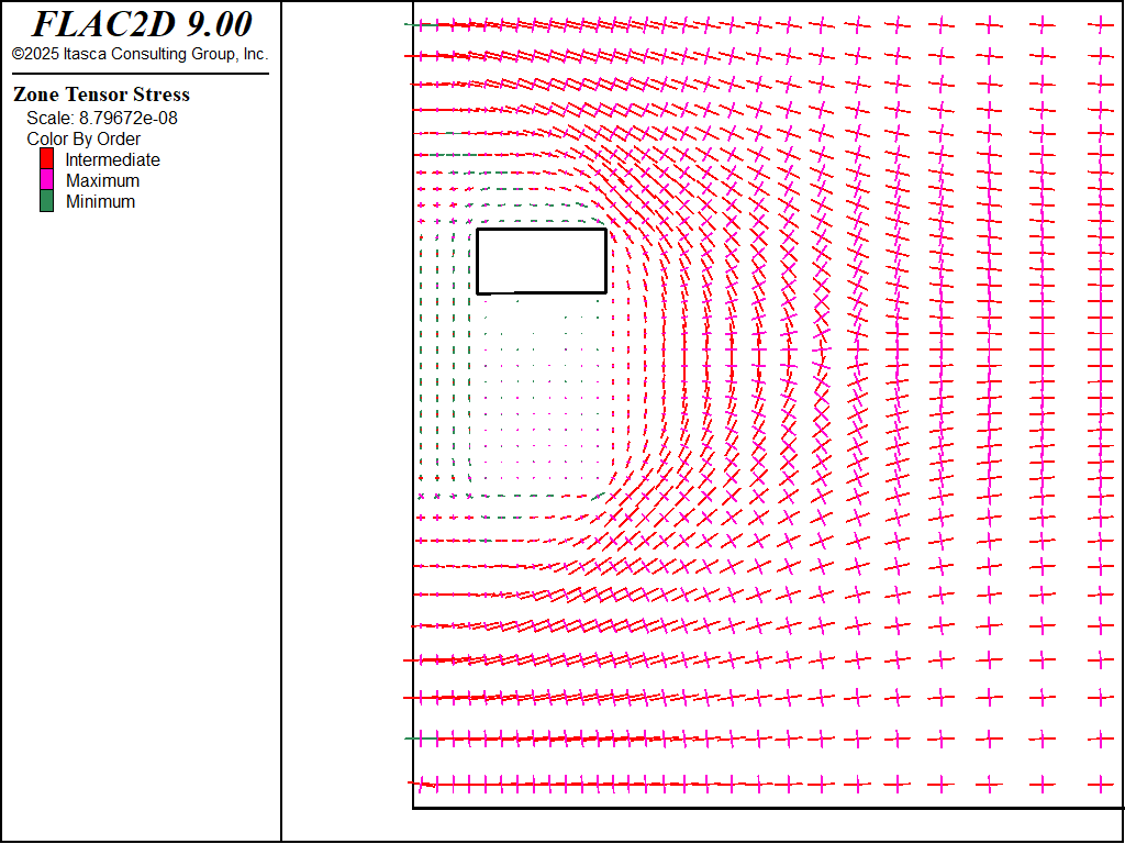
Figure 7: Principal stresses after fourth cut and fill of third cut (M-C sandfill).

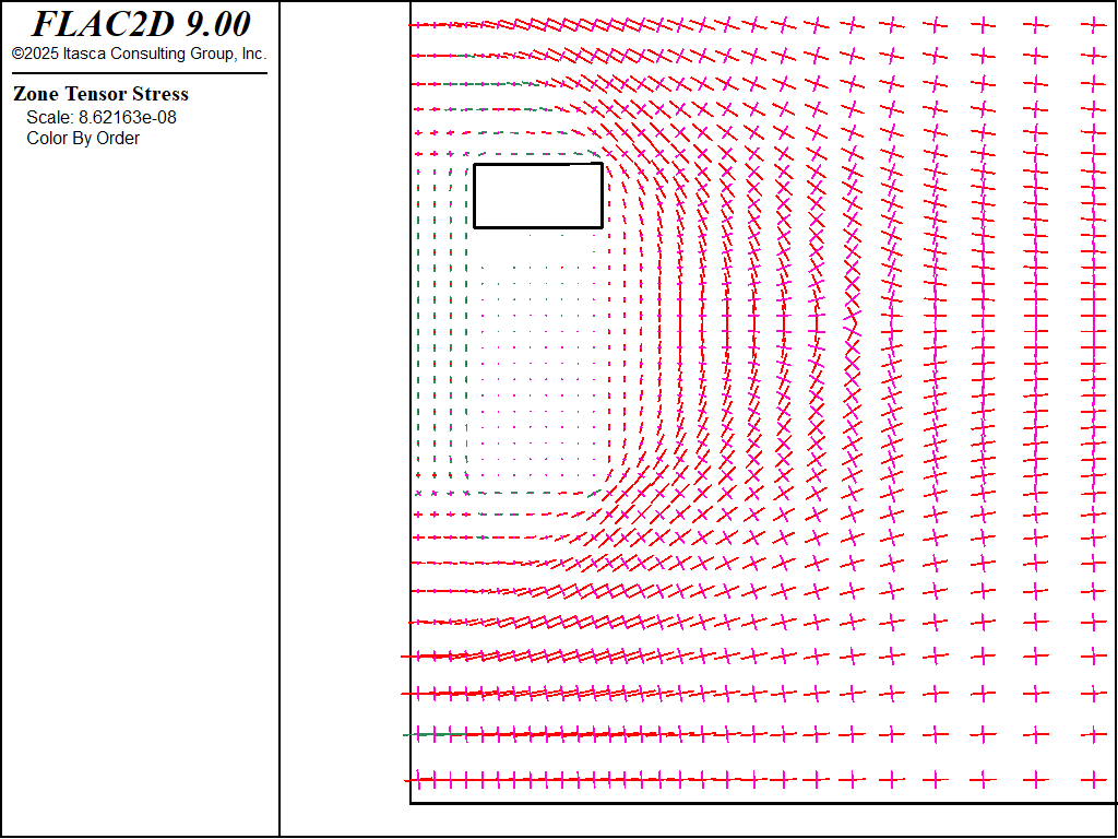
Figure 8: Principal stresses after fifth cut and fill of fourth cut (M-C sandfill).

The difference between the runs with two models can be appreciated by comparing the vertical heave in the fill. For the Mohr-Coulomb model, a maximum displacement of 9.8 cm is calculated after the fifth cut-and-fill (Figure 9). For the double-yield model, the sandfill heaves approximately 9 cm at the final stage (Figure 10). Note also that the displacement pattern is different, with more upward heave observed after each excavation stage in the Mohr-Coulomb model. This difference is due to the ability of the fill to compact using the double-yield model.

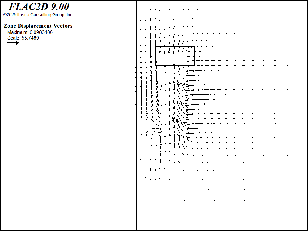
Figure 9: Displacement of fill after fifth cut, using the Mohr-Coulomb model for the sandfill.

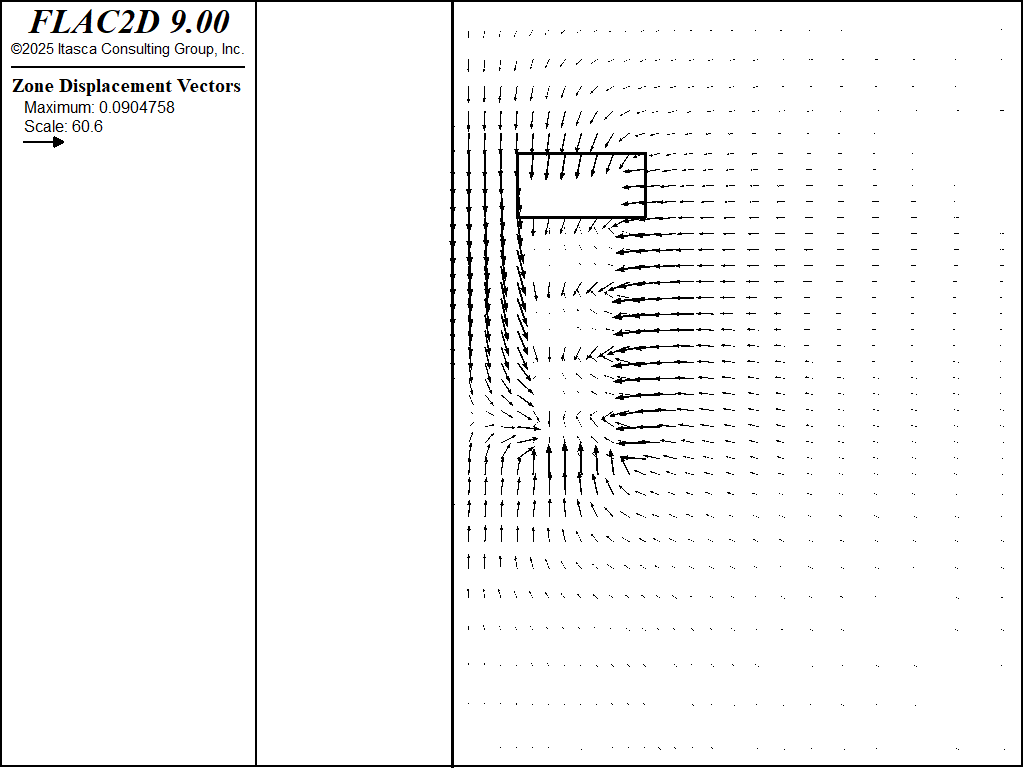
Figure 10: Displacement of fill after fifth cut, using the double-yield model for the sandfill.

The plots of the plasticity state in Figures 11 through 15 show that the pillar yields adjacent to the cut-and-fill stope, but eventually stabilizes due to the surrounding fill. Figure 16 presents a plot of horizontal displacement histories at different locations along the pillar, also indicating that the pillar is stable. For these plots, the Mohr-Coulomb model was used for the sandfill.

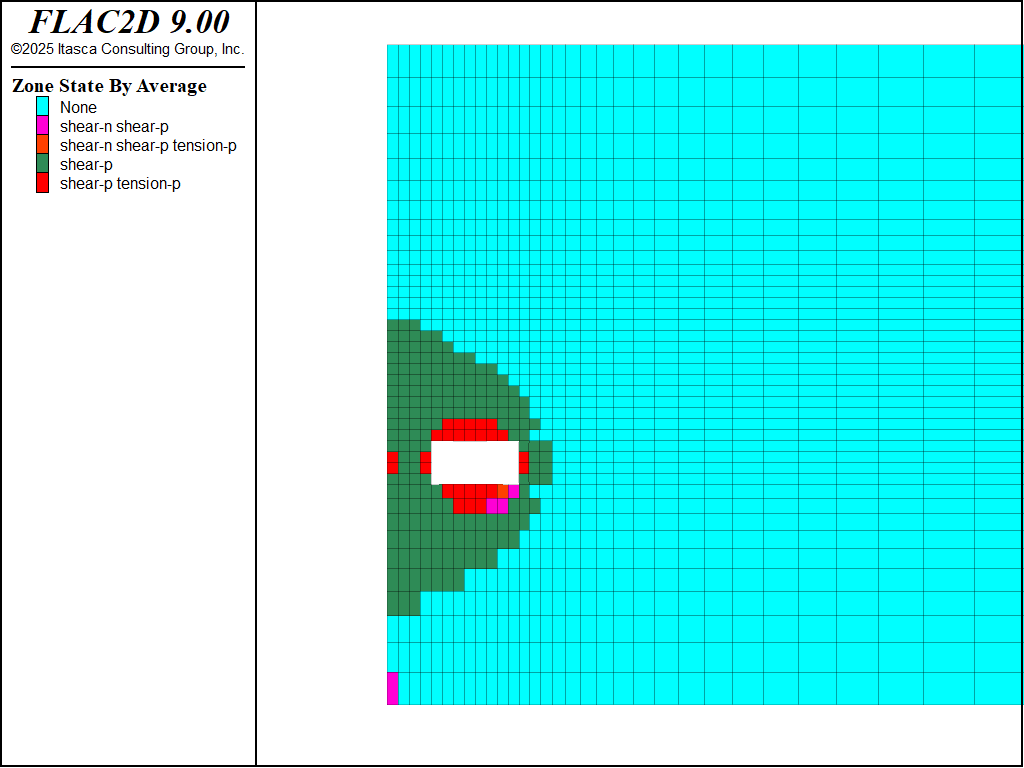
Figure 11: Plasticity state after first cut.

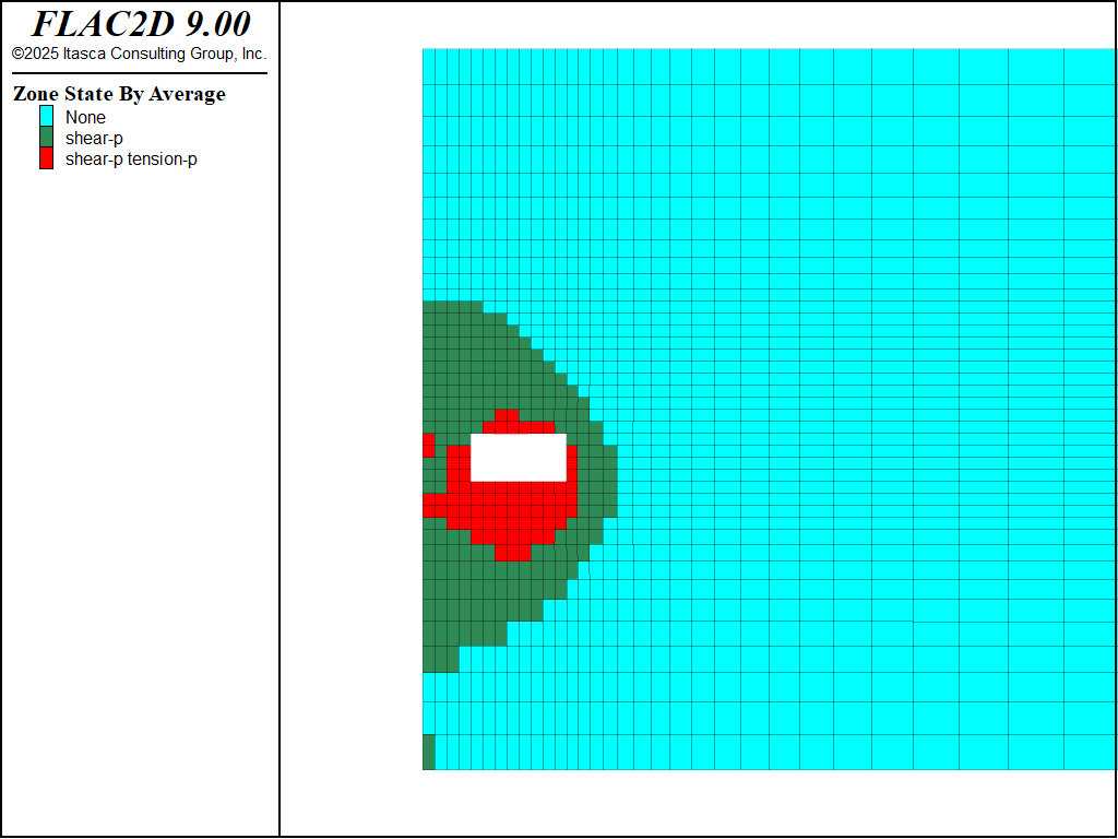
Figure 12: Plasticity state after second cut and fill of first cut (M-C sandfill).

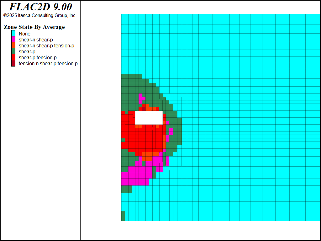
Figure 13: Plasticity state after third cut and fill of second cut (M-C sandfill).

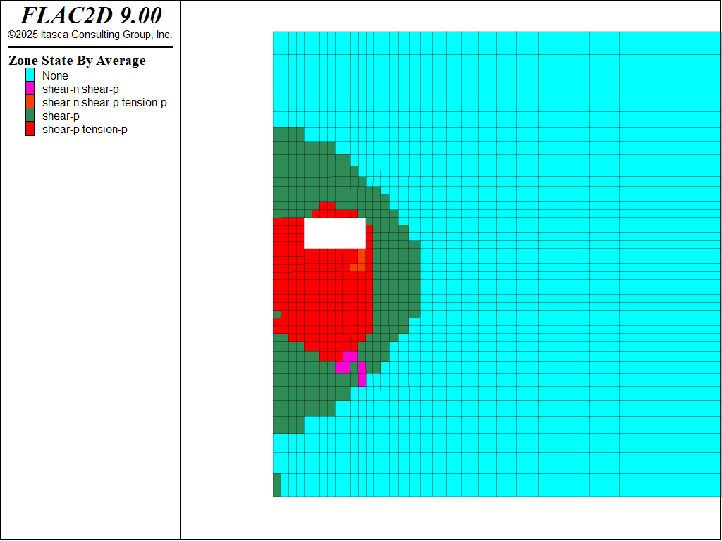
Figure 14: Plasticity state after fourth cut and fill of third cut (M-C sandfill).

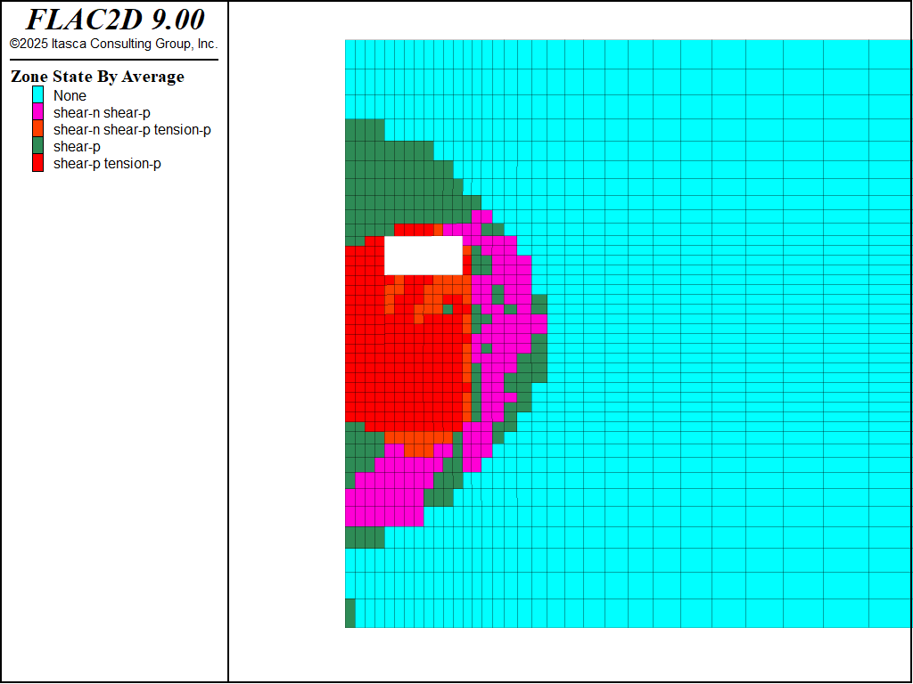
Figure 15: Plasticity state after fifth cut and fill of fourth cut (M-C sandfill).

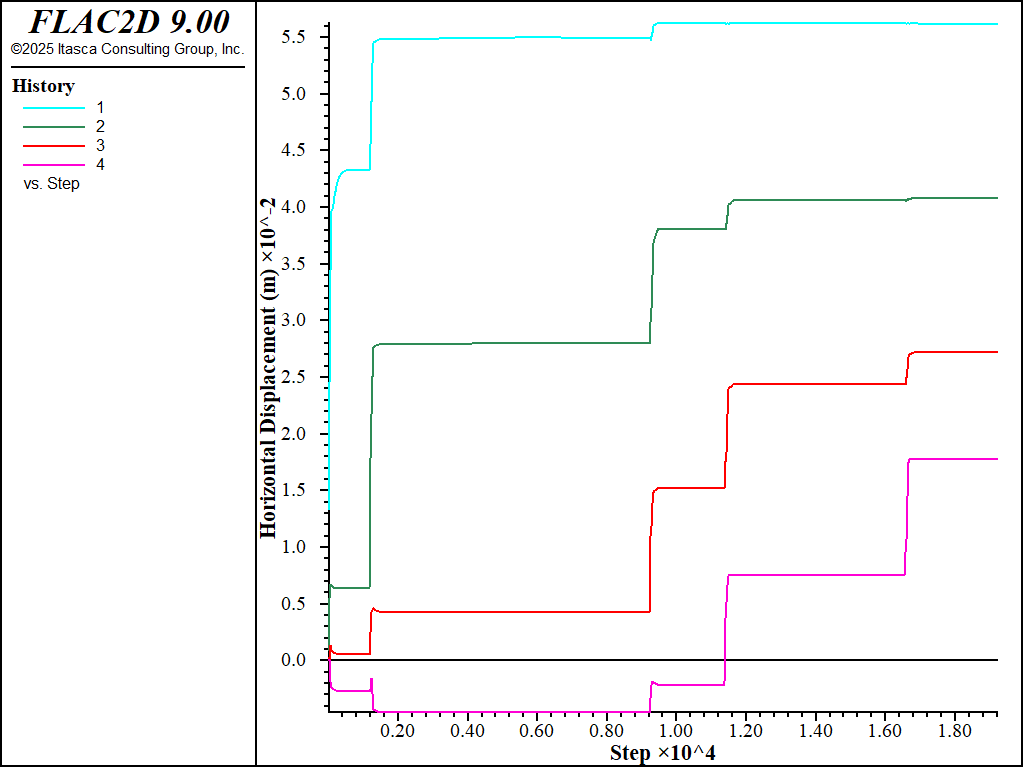
Figure 16: History of horizontal displacements at different locations along pillar (M-C sandfill).

Data File

excavate.dat

model new
model configure axisymmetry

program call 'geometry'

; properties
zone cmodel assign mohr-coulomb
zone property density 2500 bulk 1.9e10 shear 1.4e10 cohesion 3e6 ...
              friction 30 flag-brittle on

; initial and boundary conditions
zone initialize stress xx -4.5e7 yy -3e7 zz -4.5e7
zone face skin
zone face apply stress-normal -4.5e7 range group 'East'
zone face apply stress-normal -3e7 range group 'Top' or 'Bottom'

; histories
zone history displacement-x position 10 55
zone history displacement-x position 10 65
zone history displacement-x position 10 75
zone history displacement-x position 10 85

model large-strain on
model solve convergence 1

model save 'initial'

=================================================

zone cmodel assign null range group 'ex1'

model solve convergence 1

model save 'ex1'

backfill-mc.dat

model restore 'ex1'

zone cmodel assign mohr-coulomb range group 'ex1'
zone property density 1600 bulk 1e8 shear 3e7 friction 35 range group 'ex1'
zone property cohesion 500 tension 50 range group 'ex1'

zone cmodel null range group 'ex2'

model solve convergence 1

model save 'mc2'

==================================================

zone cmodel assign mohr-coulomb range group 'ex2'
zone property density 1600 bulk 1e8 shear 3e7 friction 35 range group 'ex2'
zone property cohesion 500 tension 50 range group 'ex2'

zone cmodel null range group 'ex3'

model solve convergence 1

model save 'mc3'

==================================================

zone cmodel assign mohr-coulomb range group 'ex3'
zone property density 1600 bulk 1e8 shear 3e7 friction 35 range group 'ex3'
zone property cohesion 500 tension 50 range group 'ex3'

zone cmodel null range group 'ex4'

model solve convergence 1

model save 'mc4'

==================================================

zone cmodel assign mohr-coulomb range group 'ex4'
zone property density 1600 bulk 1e8 shear 3e7 friction 35 range group 'ex4'
zone property cohesion 500 tension 50 range group 'ex4'

zone cmodel null range group 'ex5'

model solve convergence 1

model save 'mc5'

==================================================

backfill-dy.dat

model restore 'ex1'

zone cmodel assign double-yield range group 'ex1'
zone property density 1600 bulk 1e8 shear 3e7 bulk-maximum 1e8 shear-maximum 3e7  ...
  friction 35 cohesion 500 tension 50 table-pressure-cap '1' range group 'ex1'

table '1' add 0,1E4 0.02,2E5 0.04,8E5 0.06,1.3E6 0.08,3.5E6 0.1,5.5E6 0.12,8.5E6 ...
  0.14,1.15E7 0.16,1.9E7 0.18,3.4E7 0.2,5E7

zone cmodel null range group 'ex2'

model solve convergence 1

model save 'dy2'

==================================================

zone cmodel assign double-yield range group 'ex2'
zone property density 1600 bulk 1e8 shear 3e7 bulk-maximum 1e8 shear-maximum 3e7  ...
  friction 35 cohesion 500 tension 50 table-pressure-cap '1' range group 'ex2'

zone cmodel null range group 'ex3'

model solve convergence 1

model save 'dy3'

==================================================

zone cmodel assign double-yield range group 'ex3'
zone property density 1600 bulk 1e8 shear 3e7 bulk-maximum 1e8 shear-maximum 3e7  ...
  friction 35 cohesion 500 tension 50 table-pressure-cap '1' range group 'ex3'

zone cmodel null range group 'ex4'

model solve convergence 1

model save 'dy4'

==================================================

zone cmodel assign double-yield range group 'ex4'
zone property density 1600 bulk 1e8 shear 3e7 bulk-maximum 1e8 shear-maximum 3e7  ...
  friction 35 cohesion 500 tension 50 table-pressure-cap '1' range group 'ex4'

zone cmodel null range group 'ex5'

model solve convergence 1

model save 'dy5'

==================================================

Endnotes

[1]

To view this project in FLAC2D, use the program menu.

Help ▼ Examples…

  ⮡   FLAC
   ⮡   Example Applications
    ⮡   FromFLAC
     ⮡   02PostPillarMining
     ⮡   postpillar.prj