Brazilian Test (FLAC2D)

Problem Statement

Note

The project file for this example is available to be viewed/run in FLAC2D.[1] The main data files used are shown at the end of this example.

The Brazilian test (see Goodman 1980, for example) is used to estimate the tensile strength of rock and concrete. A disk or cylinder of the material is loaded diametrically between the platens of a testing machine. The specimen typically fails by developing an extension fracture along the loaded diameter. The Brazilian tensile strength is estimated from the test result by reporting the horizontal stress, \(σ_t\) (i.e., the stress perpendicular to the loaded diameter along the center part of the specimen), that corresponds to the applied compression load. The relation between \(σ_t\) and the applied load can be determined approximately from an analytical expression, assuming that the material is homogeneous, linearly elastic, and isotropic. This verification test compares the FLAC2D calculation to this solution.

The Brazilian test is only valid if the primary fracture initiates from the center of the specimen and spreads along the loaded diameter (which dictates the configuration of the numerical grid). The FLAC2D analysis can also study the test conditions that affect fracture initiation. In this example, the influence of the size of the loading area of the platen is evaluated. The parameters describing the problem conditions are shown in Figure 1. The loading area is defined by \(2α\), which is the angular distance over which the applied force, \(F\), is assumed to be distributed radially. \(r_o\) is the radius of the specimens.

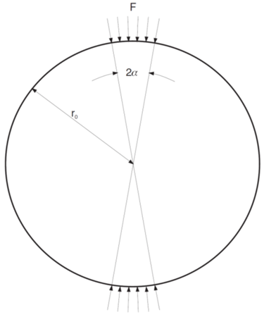
Figure 1: The Brazilian test configuration.

Analytical Solution

The stress component normal to the loading diameter, \(σ_θ\), and the stress component along the loading diameter, \(σ_r\), are given by the expressions (see Vutukuri et al. 1974).

\[\begin{split}\begin{align} \sigma_{\theta } =& + \frac{F}{\pi r_o t \alpha}\left [\frac{ \left( 1 - \left(\frac{r}{r_o}\right)^2 \right) \sin 2 \alpha}{1 -2\left(\frac{r}{r_o}\right)^2 \cos 2\alpha + \left(\frac{r}{r_o}\right)^4} - \tan^{-1}\left(\frac{1 + \left(\frac{r}{r_o}\right)^2}{1- \left(\frac{r}{r_o}\right)^2} \tan\alpha \right) \right ] \\ \\ \sigma_r =& - \frac{F}{\pi r_o t \alpha}\left [\frac{ \left( 1 - \left(\frac{r}{r_o}\right)^2 \right) \sin 2 \alpha}{1 -2\left(\frac{r}{r_o}\right)^2 \cos 2\alpha + \left(\frac{r}{r_o}\right)^4} + \tan^{-1}\left(\frac{1 + \left(\frac{r}{r_o}\right)^2}{1- \left(\frac{r}{r_o}\right)^2} \tan\alpha \right) \right ] \end{align}\end{split}\]

where \(t\) is the thickness of the cylindrical specimen and \(r\) is the distance from the center of the specimen. (Compressive stress is negative.)

The value of \(σ_θ\) at the center of the cylinder is

\[\sigma^c_\theta = \frac{F}{\pi r_o t} \left[ \frac{\sin 2\alpha}{\alpha} -1 \right] \approx \frac{F}{\pi r_o t}\]

This approximation is used to calculate the tensile strength, \(σ_t\). It is assumed that failure is independent of stresses that develop normal to the disk face and is a plane-strain solution.

FLAC2D Model

The model for the FLAC2D analysis of the Brazilian test represents a cylindrical specimen with a radius, \(r_o\), of 20 m and a thickness, \(t\) , of 1 m. Only the top half of the cylinder is modeled because of the symmetry of the Brazilian test. Figure 2 shows the FLAC2D grid. The strain-softening material model is used to simulate the behavior of the specimen. The elastic material properties and mass density assigned to the specimen are

density (\(ρ\))	2500 kg/m3
shear modulus (\(G\))	1.0 GPa
bulk modulus (\(K\))	3.0 GPa

The strength properties assigned to the strain-softening model are

cohesion (\(c\))	3.0 MPa
friction angle (\(φ\))	45
dilation angle (\(ψ\))	0
tensile strength (\(σ_t\))	1.0 MPa

The material is considered brittle with a total loss of cohesion at a plastic shear strain of \(10^{(-6)}\), and a total loss of tensile strength at a plastic tensile strain of \(10^{(-6)}\).

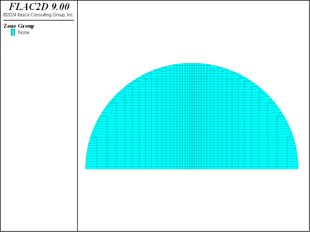
Figure 2: FLAC2D grid for Brazilian test.

The zone face apply stress-normal command is used to apply the diametrical load as a normal stress. The boundary over which the pressure is applied is selected to correspond to the loading area defined by 2α. Two cases of loading area are studied: Case 1 corresponds to \(2α ≈13^°\); and Case 2 corresponds to \(2α ≈5^°\). The applied normal stress increases at a rate of 1.0 kPa per step. The load is increased to a level that is a few steps below the load at which failure initiates. The boundary conditions and applied forces for Case 1 at a normal stress of 14.244 MPa are shown in Figure 3. A FISH function, load, calculates the applied load, \(F\), and the horizontal stress, \(σ_θ^c\), at the center of the specimen. The analytical expressions are input in tables (11 and 12 in the data file) with the FISH function braz_analytical, and the FLAC2D results for \(σ_r\) and \(σ_θ\) through the specimen are stored in tables (21 and 22 in the data file) via the FISH function braz_num, for comparison purposes.

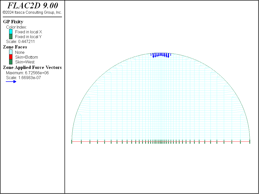
Figure 3: Boundary conditions and applied load.

Results

The FLAC2D values for \(σ_r\) and \(σ_θ\) along the loading diameter are compared to the analytical solution in Figure 4 for Case 1 and in Figure 5 for Case 2. In both cases the agreement is very good. The failure mode is very different for each case. In Case 1, for the wider loading area, tensile failure initiates in the center of the cylinder and propagates upward, as shown in Figure 6. In Case 2, shear failure initiates first at the base of the applied load, and then shear and tensile failure propagate downward toward the center of the specimen. This is shown in Figure 7. For further discussion on the influence of loading area on the mode of failure, see Vutukuri et al. (1974).

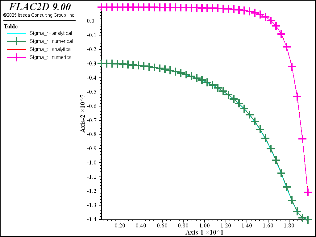
Figure 4: Comparison of \(σ_r\) and \(σ_θ\) for Case 1.

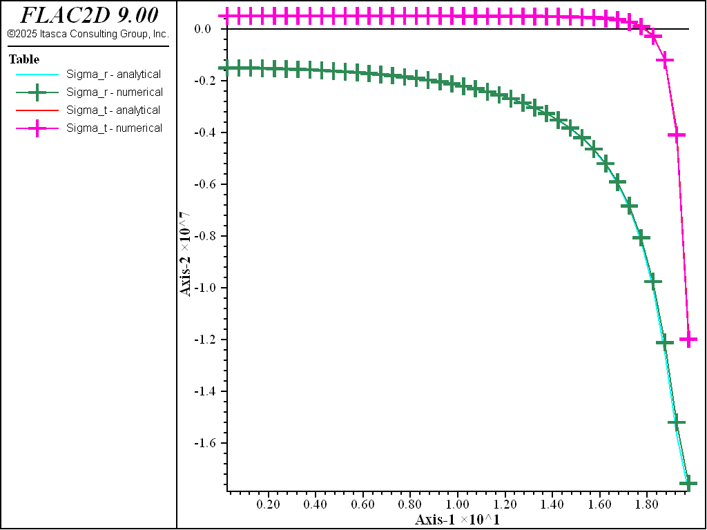
Figure 5: Comparison of \(σ_r\) and \(σ_θ\) for Case 2.

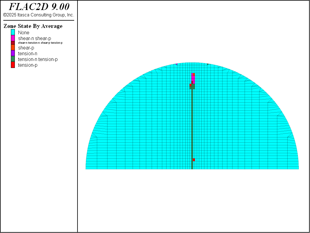
Figure 6: Initial plasticity state for Case 1.

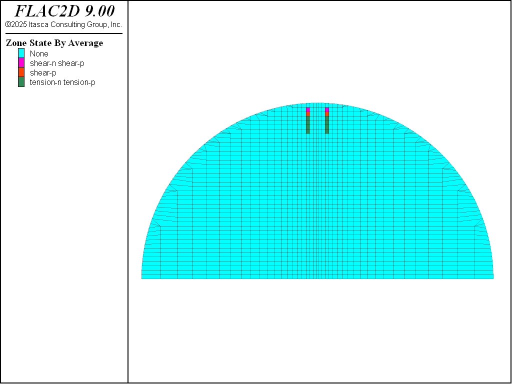
Figure 7: Initial plasticity state for Case 2.

References

Goodman, R. E. Introduction to Rock Mechanics. New York: John Wiley & Sons (1980).

Vutukuri, V. S., R. D. Lama and S. S. Saluja. Handbook on Mechanical Properties of Rocks, Vol. 1. Clausthal, Germany: Trans Tech. (1974).

Data Files

case1.dat

;------------------------------------------------------------------------------
;The Brazilian test is used to estimate the tensile strength of rock and 
;concrete. A disk or cylinder of the material is loaded diametrically between
;the platens of a testing machine.The boundary over which the pressure is 
;applied is selected to correspond to the loading area defined by 2α.
;Two cases of loading area are studied: 

;Case 1 corresponds to 2α ≈ 13 degree 
;------------------------------------------------------------------------------

model new
model large-strain off
model configure
; Create zones
zone import 'grid'
; Assign constitutive model and properties 
zone cmodel assign strain-softening
zone property bulk 3.e9 shear 1.e9 density 2500 ...
              friction 45 cohesion 3.e6 tension 1.e6 dilation 5
zone property table-cohesion '1' table-tension '2'
table '1' add (0.0,3.e6),(1.e-6,0),(1.0,0.0)
table '2' add (0.0,1.0e6),(1.e-6,0),(1.0,0.0)
zone face skin
; Boundary Conditions
zone gridpoint fix velocity-y range group 'Bottom'
[pnt = list(gp.list)(gp.isgroup(::gp.list,"Bottom"))]

fish define parm_case1
    global alfa = math.atan(2.2515/19.873) ; corresponds to i=27 j=41 in old FLAC
    global ang_factor = math.sin(2.0*alfa)/alfa-1.0
end
[parm_case1]

;define load
fish define load
    local sum= 0.0
    sum = -1.0*list.sum(gp.force.unbal(::pnt)->y)
    load=sum
    global sigma_t = sum*ang_factor/(20.0*math.pi)
end

; Analytical solution
fish define braz_analytical
    local rad0 = 20.0
    local app_str = float(global.step) * 1000.0
    local app_for = 2.0 * app_str * rad0 * alfa    
    loop local jj (1,40)
        local rad = 0.25 + (float(jj-1) * 0.5)
        local radrat = rad / rad0
        local for_den = math.pi * rad0 * alfa
        local t1_t = (1.0 - (radrat)^2) * math.sin (2.0 * alfa)
        local t1_b = 1.0 - (2.0 * (radrat)^2 * math.cos(2.0*alfa)) + (radrat)^4
        local t2_t = (1.0 + (radrat)^2) / (1.0 - (radrat)^2)
        local t2_b =  math.tan(alfa)
        local t2_tb = t2_t * t2_b
        local t2   = math.atan(t2_tb)
        local sigma_t =   (app_for / for_den) * ((t1_t / t1_b) - t2)
        local sigma_r = - (app_for / for_den) * ((t1_t / t1_b) + t2)
        table.x(11,jj) = rad
        table.y(11,jj) = sigma_t
        table.x(12,jj) = rad
        table.y(12,jj) = sigma_r
    end_loop
end

;Numerical results from FLAC2D
fish define braz_num
    local vl= (-.15,0.0)
    local vu= (.15, 20.0)
    local zlist = zone.inbox(vl,vu,false)
    local jj=1    
    loop foreach local pnt zlist
        local rad = 0.25 + (float(jj-1) * 0.5)
        table.x(21,jj) = rad
        table.y(21,jj) = zone.stress.xx(pnt)
        table.x(22,jj) = rad
        table.y(22,jj) = zone.stress.yy(pnt)
        jj=jj+1
    end_loop
end
;
;define loading ramp
fish define loading_ramp
    loading_ramp= global.step
end

zone face apply stress-normal -1.0e3 fish loading_ramp ...
                range position-y 19.870 20
history interval 10
model history mechanical unbalanced-maximum
zone history stress quantity xx position (-0.496,0.0)
zone history stress quantity yy position (-0.496,0.0)
zone history stress quantity xx position (-0.496,19.5)
zone history stress quantity yy position (-0.496,19.5)
zone history stress quantity xx position (-0.09,0.01)
fish history load
fish history sigma_t
fish history loading_ramp
model large-strain off
model step 14000
[braz_analytical]
[braz_num]
model save 'case1'
model step 300
model save 'case1f'

case2.dat

;------------------------------------------------------------------------------
;Case 2 corresponds to 2α=5 degree
;------------------------------------------------------------------------------

model new
model large-strain off
model configure
; Create zones
zone import 'grid'
; Assign constitutive model and properties 
zone cmodel assign strain-softening
zone property bulk 3.e9 shear 1.e9 density 2500 ...
              friction 45 cohesion 3.e6 tension 1.e6 dilation 5
zone property table-cohesion '1' table-tension '2'
table '1' add (0.0,3.e6),(1.e-6,0),(1.0,0.0)
table '2' add (0.0,1.0e6),(1.e-6,0),(1.0,0.0)
zone face skin
; Boundary Conditions
zone gridpoint fix velocity-y range group 'Bottom'
[pnt = list(gp.list)(gp.isgroup(::gp.list,"Bottom"))]

;define angle
fish define parm_case2
    global alfa=math.atan(0.87696/19.981) ; corresponds to i=24 j=41 in old FLAC
    global ang_factor=math.sin(2.0*alfa)/alfa-1.0
end
[parm_case2]

;define load
fish define load
    local sum= 0.0
    sum = -1.0*list.sum(gp.force.unbal(::pnt)->y)
    load=sum
    global sigma_t=sum*ang_factor/(20.0*math.pi)
end

; Analytic solution
fish define braz_analytical
    local rad0 = 20.0
    local app_str = float(global.step) * 1000.0
    local app_for = 2.0 * app_str * rad0 * alfa        
    loop local jj (1,40)
        local rad = 0.25 + (float(jj-1) * 0.5)
        local radrat = rad / rad0
        local for_den = math.pi * rad0 * alfa
        local t1_t = (1.0 - (radrat)^2) * math.sin (2.0 * alfa)
        local t1_b = 1.0 - (2.0 * (radrat)^2 * math.cos(2.0*alfa)) + (radrat)^4
        local t2_t = (1.0 + (radrat)^2) / (1.0 - (radrat)^2)
        local t2_b =  math.tan(alfa)
        local t2_tb = t2_t * t2_b
        local t2   = math.atan(t2_tb)
        local sigma_t =   (app_for / for_den) * ((t1_t / t1_b) - t2)
        local sigma_r = - (app_for / for_den) * ((t1_t / t1_b) + t2)
        table.x(11,jj) = rad
        table.y(11,jj) = sigma_t
        table.x(12,jj) = rad
        table.y(12,jj) = sigma_r
    end_loop
end

;Numerical results from FLAC2D
fish define braz_num
    local vl= (-.15,0.0)
    local vu= (.15, 20.0)
    local zlist = zone.inbox(vl,vu,false)
    local jj=1
    loop foreach local pnt zlist
        local rad = 0.25 + (float(jj-1) * 0.5)
        table.x(21,jj) = rad
        table.y(21,jj) = zone.stress.xx(pnt)
        table.x(22,jj) = rad
        table.y(22,jj) = zone.stress.yy(pnt)
        jj=jj+1
    end_loop
end

fish define loading_ramp
    loading_ramp= global.step
end

zone face apply stress-normal -1.0e3 fish loading_ramp ...
                range position-y 19.98 20
history interval 10
model history mechanical unbalanced-maximum
zone history stress quantity xx position (-0.496,0.0)
zone history stress quantity yy position (-0.496,0.0)
zone history stress quantity xx position (-0.496,19.5)
zone history stress quantity yy position (-0.496,19.5)
zone history stress quantity xx position (-0.09,0.01)
fish history load
fish history sigma_t
fish history loading_ramp
model large-strain off
model step 18000
[braz_analytical]
[braz_num]
model save 'case2'
model step 400
model save 'case2f'

Endnote

[1]

This example is listed under the present document title in the i Examples dialog (use the menu command Help -> Examples… to access).