Using the Rigid Body Spring Network Paradigm
Problem Statement
Note
The project file for this example may be viewed/run in PFC.[1] The data files used are shown at the end of this example.
As shown in the “Rigid Block Model of Tunnel Excavation” example, rigid blocks can successfully simulate the response of blocky systems where breakage occurs between blocks. Using the standard contact models in Bonded Block Models (BBM), the elastic properties must be calibrated. In addition, there is some degree of heterogeneity of elastic response, at the scale of a few rigid blocks, due to the approximate methods used to set the contact stiffnesses. The degree of heterogeneity is dependent in a complex fashion on the rigid block geometries. Achieving a very high ratio of UCS to direct tensile strength may also be challenging, and tensile damage may be unrealistic in certain scenarios due to the degree of small-scale elastic heterogeneity.
The Rigid Body Spring Network (RBSN) model, proposed by [Bolander1998a], addresses these issues. In this model, the Young’s modulus and Poisson’s ratio are specified for a bonded specimen and the elastic response is quite close to the values set, regardless of rigid block geometry used. This is accomplished using a theoretical method to set the contact stiffnesses based on a lattice with zero Poisson’s ratio. Poisson’s effect is simulated by applying an elastic correction to the contact forces, as discussed in the “Spring Network Model” description. [Rasmussen2021a] presents a thorough discussion of results for 2D Voronoi packings, along with a suggested calibration method. In this example the capabilities of this model will be demonstrated in large strain with various rigid block geometries. In this example the contact strengths and elastic constants are kept primarily uniform. To our knowledge, this is the first demonstration of the applicability of the RBSN approach where the underlying geometries vary from Voronoi packings.
Geometry Creation
This example demonstrates three methods to create rigid block packings directly inside the code. When creating rigid blocks based on a meshing method, the suggested approach is to generate the rigid blocks within a parallelepiped region larger than the final specimen size. Subsequently, the rigid blocks are trimmed to match the specimen boundaries via the rblock cut command. This is important in BBM simulations because meshing directly to the specimen boundaries may result in preferential interlocking of rigid blocks near the boundaries due to the algorithmic details of the mesh production. When using a densification approach, on the other hand, this trimming step is not necessary. With the addition of rigid block facet groups, facets cut using the group-facets keyword are easily identified. Facet groups are very helpful for applying boundary conditions and contact model properties. Note that in all examples slivers produced by the cutting algorithm are not removed.
In this example, the first packing of rigid blocks is built using the rblock construct command. The resulting {triangles in 2D; tetrahedra in 3D} form a zero-porosity representation of the parallelepiped that conforms to the boundary—with specified maximum edge length. Random perturbations to the edge lengths are prescribed via geometry node extra variables using the rblock.construct.internal keyword. This is an important part of the procedure. Without the variation in edge length, the resulting rigid blocks are nearly equidimensional, forming a rather crystalline structure. The failure characteristics of crystalline packings differ substantially from those with more randomized packings.
The second rigid block packing is a Voronoi packing. A Voronoi tessellation is created with the rblock construct from-balls command. An initial packing of balls is created with the ball generate command to provide seed positions and weights for the Voronoi construction. The balls are not cycled and are deleted after construction.
The final rigid block geometry uses the rblock densify command. The initial parallelepiped rigid block is cut to the shape of the specimen and then densification is applied to this block. Densification is a recursive cutting procedure where cuts go through the rigid block centroids. The orientations of the cutting planes, by default, are perpendicular to the longest direction of the rigid blocks. If no deviation in cut plane orientation is specified, a roughly cubical distribution of rigid blocks would result. In this example, some deviation is used to produce a non-blocky set of rigid blocks. Densification is an alternative and relatively simple way to create a zero-porosity packing without complex meshing procedures. A clear benefit is that no slivers are created. When merely creating a more refined set of rigid blocks to capture elastic response, this approach is a viable option.
These three geometries are shown in 3D in the figures below. Note the substantial differences in material fabric. In the densified specimen, due to the cutting algorithm, a number of throughgoing surfaces exist. Such coherent joint surfaces are not present in the meshing approaches. By assigning groups to facets created by the first number of cuts in the densified model, different contact model properties can be assigned to the resulting contacts in order to reduce the influence of these features on the failure response.
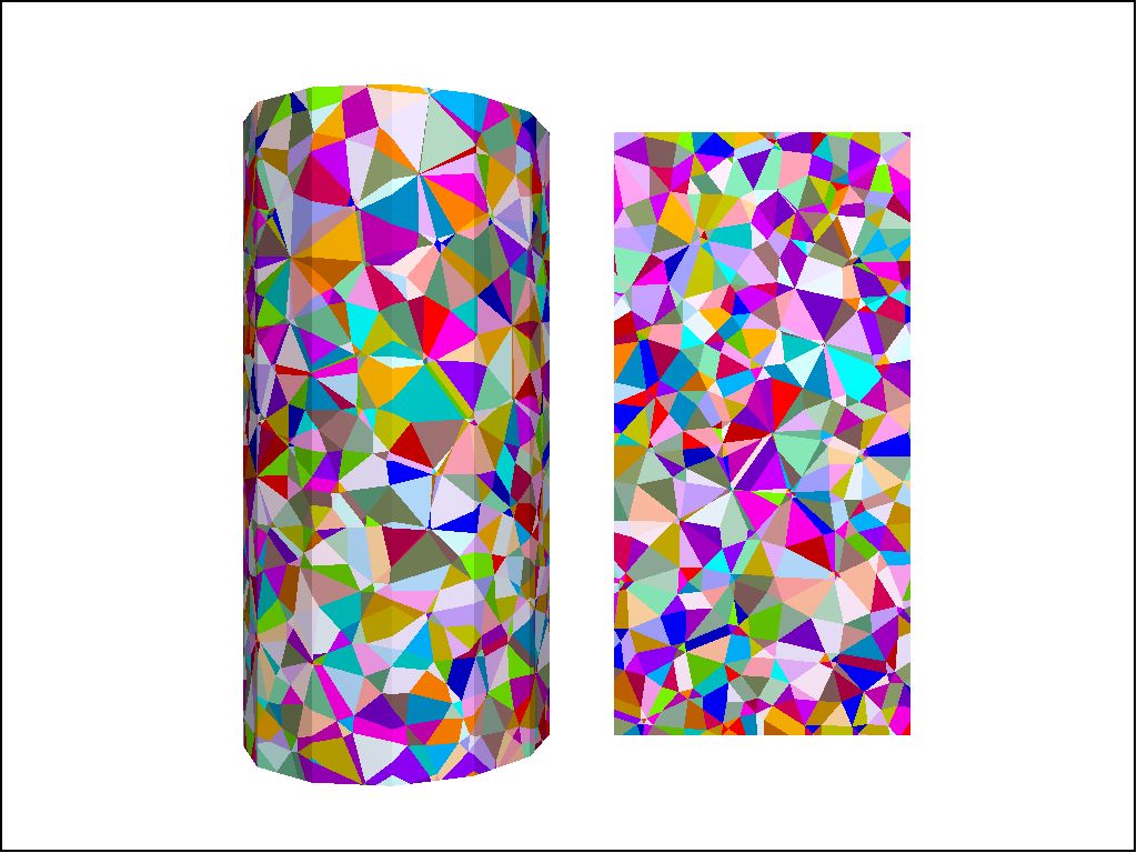
Figure 1: Tetrahedral packing with cutting plane.
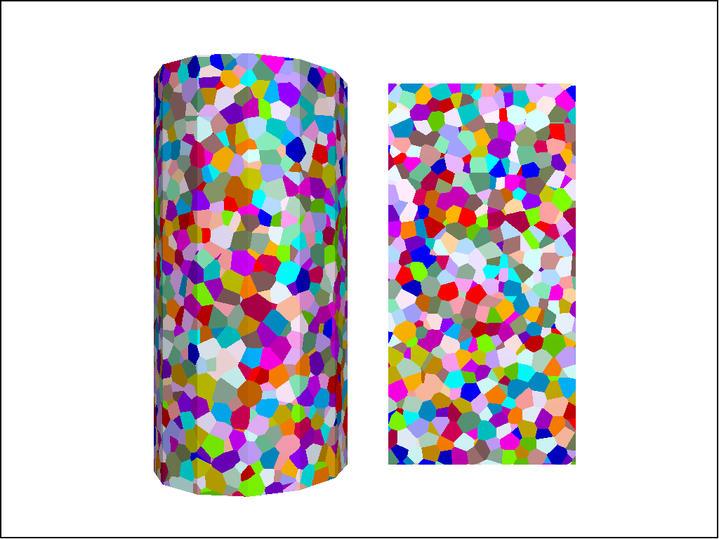
Figure 2: Voronoi packing with cutting plane.
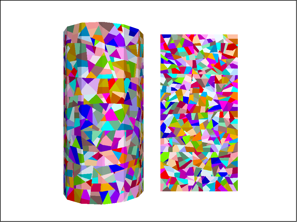
Figure 3: Densified packing with cutting plane.
Contacts
Rigid blocks must overlap initially for accurate contact detection/resolution. The rblock dilate expand command is given in this example. This is the best approach to ensure that rigid blocks in a zero-porosity packing overlap by a small amount. When using the Spring Network Model contact model, stresses must be accumulated from the contact forces during cycling. Though this operation (enabled with the rblock contact-resolution accumulate-stress command) slows cycling, the gains made by using this contact model far exceed the computational overhead. The areas must be computed from the overlap volumes as well for the stresses to be consistent with the joint areas. In order for the simulation to proceed quickly, it is important to cull edge-edge and vertex-vertex contact configurations. In this case, the rblock contact-resolution facet-total command is given so that these contacts are not created. This is acceptable for simulations involving moderate strain, and is faster and less memory intensive than inhibiting contacts.
Beyond these steps, contact model assignment is performed with the contact cmat default command and the facet groups are applied to the contacts with the rblock apply-facet-groups command. This allows setting a larger strength for the throughgoing cuts in the densified model than for the remainder of the contacts. The same method to assign contact models/properties to contacts in different regions of the model can be used. The figures below show the intact contacts plotted as joints. Though the total number of rigid blocks are ~4,000 for each geometry, the total number of contacts in each model is quite different, with about double the number of contacts in the densified and Voronoi packings as compared with the tetrahedral packing. Because computational time is directly proportional to the number of contacts, this suggests that models created from tetrahedra will run faster.
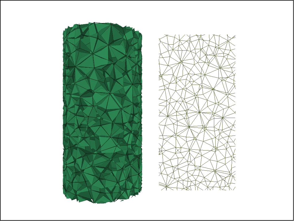
Figure 4: Contacts from the tetrahedral packing plotted as joints.
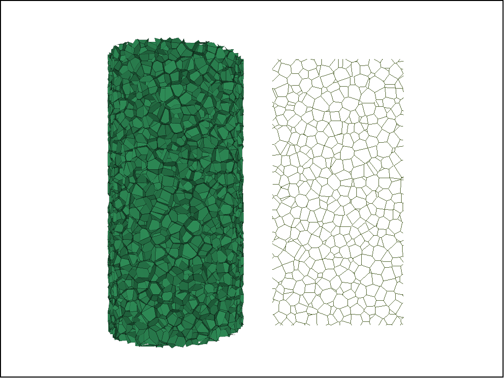
Figure 5: Contacts from the Voronoi packing plotted as joints.
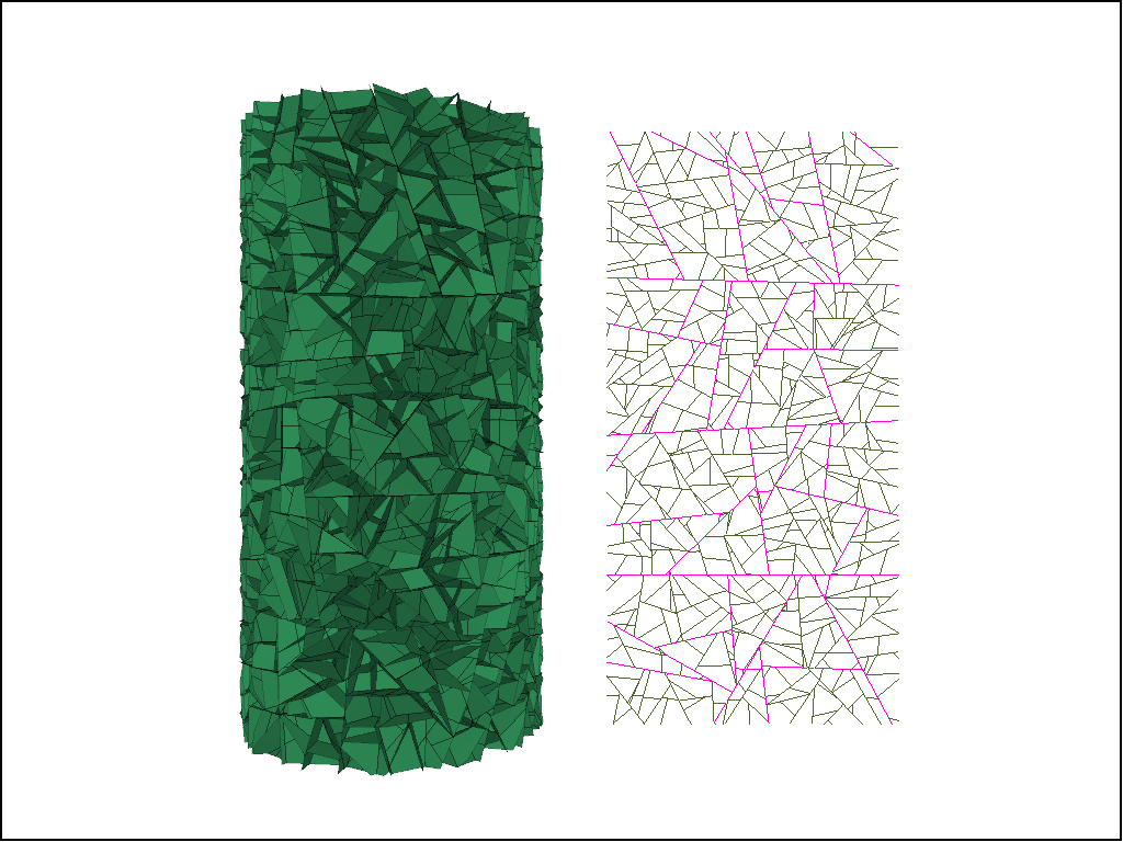
Figure 6: Contacts from the densified packing plotted as joints. The purple contacts are assigned twice the strength of the other contacts.
Testing Environment
A simple testing environment is created that runs direct tension, UCS, and { biaxial in 2D; triaxial in 3D} confinement tests. A number of measures are recorded to assess the elastic and failure responses of the materials. The Young’s modulus is approximated by the slope of the stress-strain curves, using both walls and measurement spheres. The Poisson’s ratio is estimated based on the movement of rigid blocks near the outside center of the specimens. For the confined tests, stress is applied to the outer boundaries via the rblock facet apply command. Because the timestep is scaled, it is straightforward to supply a fixed straining velocity for all specimens. By applying a velocity gradient to the rigid blocks, the initial transient response of assigning a platen velocity is substantially diminished. In the figures below the \(z\)-displacements are shown—along with failed contacts—on a wedge-shaped cutting plane through the center of the cylindrical specimen.
Direct Tension Comparisons
The figures below show comparisons of direct tension tests for the three specimens. The approximate Young’s moduli are within 5% of the specified value independent of material fabric. The estimated Poisson’s ratios are generally within ~15% of the specified value, with the densified material having the largest deviation. The finding that this RBSN implementation produces well-behaved elastic response for these various material fabrics allows for the application of this approach on a wide variety of model geometries. Note that the elastic constant values will vary slightly depending on the specific realization of any material fabric. Also note the lack of substantial damage away from the main failure surfaces. Such pre-peak damage is commonly observed in simulations with Voronoi specimen using the Soft-Bond Model model. The lack of pre-peak damage in direct tension is a clear manifestation of the diminished level of elastic heterogeneity at the rigid block scale embodied by the RBSN approach. Thus, evidence suggests that models created using the RBSN approach may produce results similar to 3DEC models composed of deformable blocks. The macro-tensile strength is ~30% lower than the specified micro-tensile strength, with the Voronoi specimen having the highest tensile strength due to the rough material fabric.
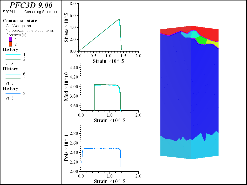
Figure 7: Direct tension test of the tetrahedral specimen.
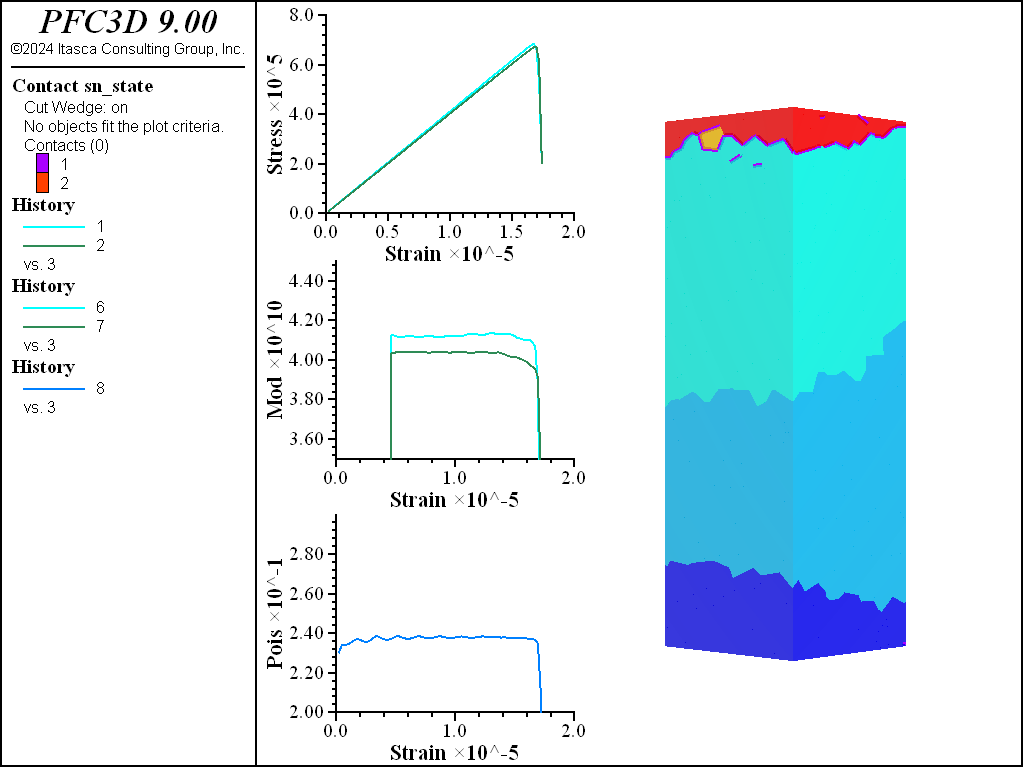
Figure 8: Direct tension test of the Voronoi specimen.
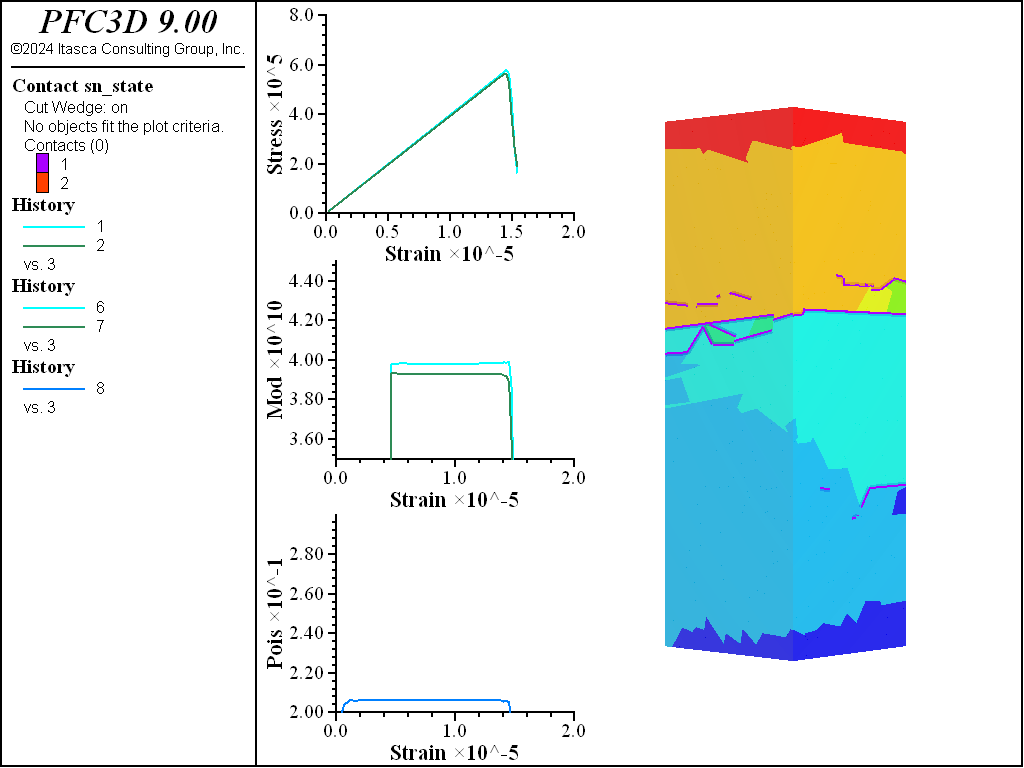
Figure 9: Direct tension test of the densified specimen.
UCS Comparisons
The figures below show the results of the UCS tests. The scales are different from the direct tension results though the slopes are kept unchanged. As with the direct tension test, the elastic properties are well represented without the need for material calibration. The micro-cohesive strength is a factor of 5 higher than the micro-tensile strength. In all cases the ratio of UCS to direct tensile strength is about 10, and the UCS results show quite brittle responses. The majority of damage comes in the form of tensile cracks with interconnecting shear cracks. Note that, once failure has initiated, the measure of Poisson’s ratio is no longer applicable.
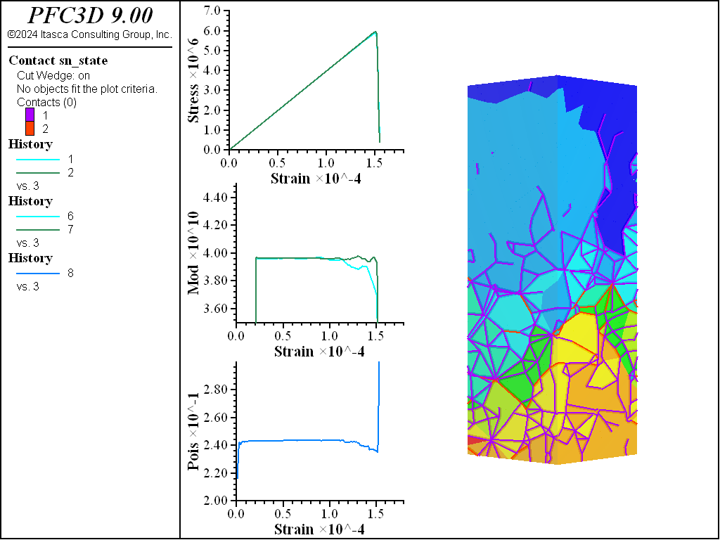
Figure 10: UCS test of the tetrahedral specimen.
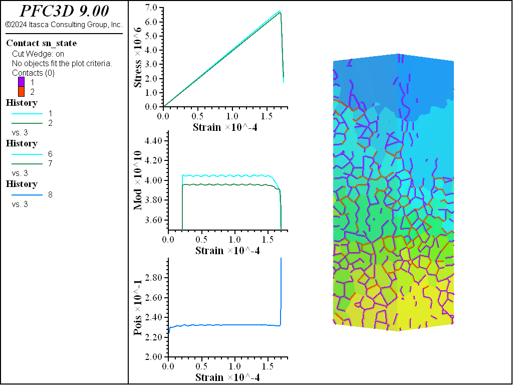
Figure 11: UCS test of the Voronoi specimen.
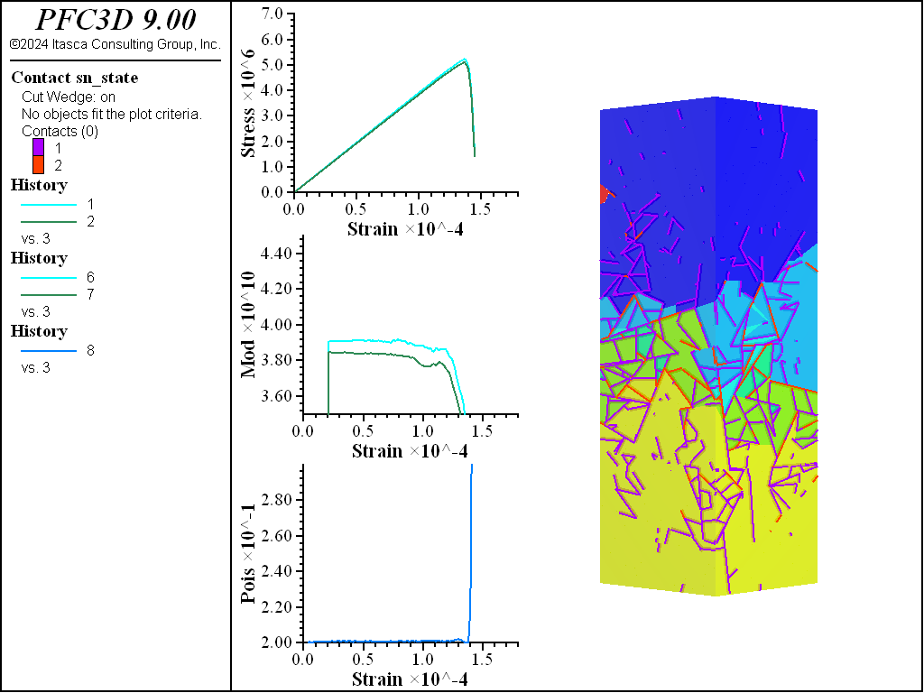
Figure 12: UCS test of the densified specimen.
Triaxial Comparisons
The figures below compare 1 MPa triaxial confinement tests. As with the unconfined tests, the elastic properties are captured well with the RBSN approach for all material fabrics. The strength does not drop to zero for any of the specimens. This is especially apparent for the Voronoi and densified models. When looking at the stress on individual rigid blocks in these models, it is clear that in a real specimen fracture would occur within the intact region. These models will not capture this response but, with the ability to cut rigid blocks and retain contacts, the failure response of the intact material could be simulated.
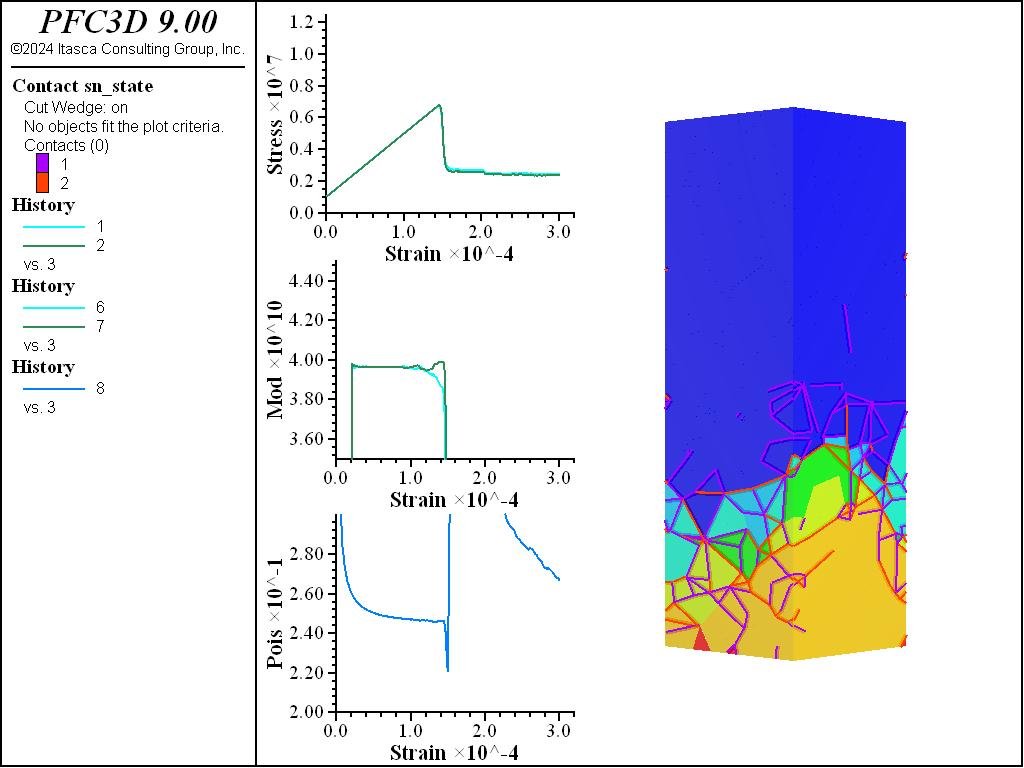
Figure 13: Triaxial test of the tetrahedral specimen.
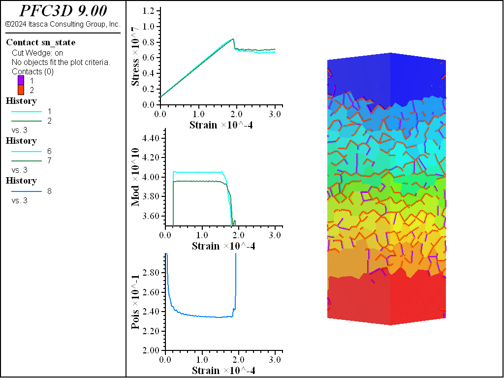
Figure 14: Triaxial test of the Voronoi specimen.
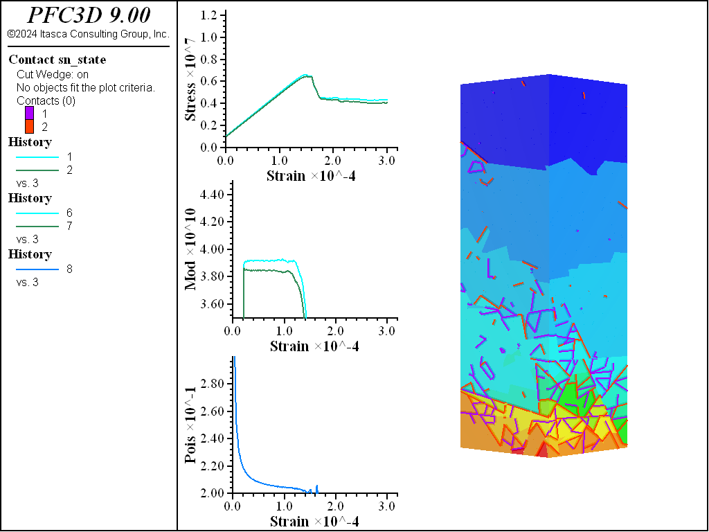
Figure 15: Triaxial test of the densified specimen.
References
Bolander, J. and Saito, S., “Fracture Analyses using Spring Networks with Random Geometrys” in Eng. Fract. Mech., 61(5), pp. 569-591, 1998.
Rasmussen, L., “Hybrid Lattice/discrete Element Method for Bonded Block Modeling of Rocks” in Computers and Geotechnics, 130, article 103907, 2021.
Data Files
step1Geometry.dat
; Example demonstrating different ways to generate rigid block
; specimen.
model new
model random 10000
; Dimensions of the final cylinder for testing.
[radius = 2.5]
[height = 10.]
model domain extent [-2*radius] [2*radius] [-2*radius] ...
                    [2*radius] [-height] [height]
; FISH function to trim the rblocks to a cylindrical container.
; It is important to create rblocks conforming to a larger
; container since meshing artifacts generally exist near the
; boundaries of the container.
fish define trim
    command
        geometry set 'container'
        geometry generate cylinder resolution 0.5 ...
            base 0 0 [-height/2.0] height [height] ...
            radius [radius]
        fracture import from-geometry 'container'
        ; Cut rblocks, keeping slivers and assigning facet groups
        ; to the boundaries for stress application.
        rblock cut fractures 'container' throughgoing ...
            sliver-remove false group-facets 'outside' slot 'outside'
        ; Assign different facet groups to the platens.
        rblock facet group 'platen' slot 'outside' ...
            range position-z [height/2.0] tolerance 1e-5
        rblock facet group 'platen' slot 'outside' ...
            range position-z [-height/2.0] tolerance 1e-5
        ; Delete all rigid blocks outside the container.
        rblock delete range geometry-space 'container' count even
        geometry delete
        fracture delete
    endcommand
end

; Specimen 1: tetrahedral packing with some random scaling inside
; the volume. The random scaling is important otherwise the fabric
; is completely crystalline.
geometry set 'blocks'
geometry generate box [-2*radius] [2*radius] ...
    [-2*radius] [2*radius] [-height] [height]
; Maximum edge length for the mesher.
[maxEdge = 0.85]
; Create geometry nodes inside the generation volume.
; Extra variables are assigned to provide random weights
; to the surface and volume mesher.
geometry fill [maxEdge]
geometry node extra 1 [maxEdge]
fish define addExtra
    local spacing = maxEdge
    local std = spacing/2.5
    local gs = geom.set.find("blocks")
    local nme = 0
    loop foreach local gn geom.node.list(gs)
        local newVal = maxEdge + ...
            (math.random.uniform() - 0.5)*2.0*std
        nme = math.max(nme,newVal)
        geom.node.extra(gn,1) = newVal
    endloop
    maxEdge = nme
end
[addExtra]
; Use the INTERNAL keyword to use the weights.
rblock construct from-geometry 'blocks' maximum-edge [maxEdge] ...
    internal
geometry delete
[trim]
model save 'tet'
rblock delete

; Specimen 2: Voronoi packing generated from balls. The balls
; act as seed points for the Voronoi mesh creation.
ball delete
ball generate number 100000 tries 1000000 radius 0.11 0.2
rblock construct from-balls polydisperse true
ball delete
[trim]
model save 'voro'
rblock delete

; Specimen 3: use the DENSIFY command to create a randomly cut specimen.
rblock create box [-2*radius] [2*radius] [-2*radius] [2*radius] ...
    [-height] [height]
; In this case trim first so that strange boundary layers can occur due
; to an initial cut0
[trim]
; Densify and assign facet groups. Densification is iterative so the
; first number of cuts span the entire model. These would represent
; large scale continuous fracture surfaces. Later we will give these more
; strength so that failure is not preferred on these surfaces.
rblock densify iterations 6 random 45 ...
    facet-group 'elastic' slot 'densify'
; Densify to a specified size.
rblock densify size 0.07 random 90
model save 'random'
step2Contacts.dat
; Create the contacts and assign the proerties.
; See contacts.dat for more information.

model restore 'tet'
[emod = 4.e+10]
[pois = 0.25]
[fric = 0.2]
[tenStr = 9.e+05]
[cohFac = 5.]
[facetTotal = 0.05]
program call 'contacts'
model save 'tetContacts'

model restore 'voro'
[emod = 4.e+10]
[pois = 0.25]
[fric = 0.2]
[tenStr = 9.e+05]
[cohFac = 5.]
[facetTotal = 0.001]
program call 'contacts'
model save 'voroContacts'

model restore 'random'
[emod = 4.e+10]
[pois = 0.25]
[fric = 0.2]
[tenStr = 9.e+05]
[cohFac = 5.]
[facetTotal = 0.001]
program call 'contacts'
model save 'randomContacts'
step3Tests.dat
; Run the tests
; See test.dat for more information.

; Direct tension
model restore 'tetContacts'
[compress = false]
[confinement = 0]
program call 'tests'
model save 'tetTen'
model restore 'voroContacts'
[compress = false]
[confinement = 0]
program call 'tests'
model save 'voroTen'
model restore 'randomContacts'
[compress = false]
[confinement = 0]
program call 'tests'
model save 'randomTen'

; UCS
model restore 'tetContacts'
[compress = true]
[confinement = 0]
program call 'tests'
model save 'tetUCS'
model restore 'voroContacts'
[compress = true]
[confinement = 0]
program call 'tests'
model save 'voroUCS'
model restore 'randomContacts'
[compress = true]
[confinement = 0]
program call 'tests'
model save 'randomUCS'

; Triaxial
model restore 'tetContacts'
[compress = true]
[confinement = -1e6]
program call 'tests'
model save 'tetTriax'
model restore 'voroContacts'
[compress = true]
[confinement = -1e6]
program call 'tests'
model save 'voroTriax'
model restore 'randomContacts'
[compress = true]
[confinement = -1e6]
program call 'tests'
model save 'randomTriax'
contacts.dat
; Create the contacts and assign the properties
; Expected input parameters are:
;   emod        Young's modulus
;   pois        Poisson ratio
;   fric        Friction coefficient
;   tenStr      Tensile strength
;   cohFac      Cohesion is set to this factor multiplied by the
;               tensile strength.

; Instead of self-similar scaling, dilation has been modified so that
; the facets are all moved outward (in the facet normal direction)
; by the specified amount
rblock dilate expand 0.0001 keep-inertial
; Set the density and use local damping
rblock attribute density 2750 damp 0.7
; The following command specifies:
;   1) Use areas in contacts for computing stiffnesses
;   2) Stress accumulation while cycling is required for the springnetwork
;      model
;   3) Do not create contacts with initial area less than 1% of the total facet
;      area. This is more efficient than inhibiting the contacts but, for very
;      large strain problems, inhibiting may be more desirable as the contacts
;      can be checked periodically for activation.
rblock contact-resolution update-area true accumulate-stress true ...
                          facet-total [facetTotal]
; Assign the springnetwork model as the default slot in the CMAT
contact cmat default model springnetwork property sn_ten 1e100 ...
                           sn_coh 1e100 fric [fric] ...
                           method compute-stiffness emod [emod] poisson [pois]
; Create the contacts
model clean all

; Apply any facet groups to contacts.
rblock apply-facet-groups

; Assign uniform tensile strength in this simple example.
contact property sn_ten [tenStr] sn_coh [tenStr*cohFac] ...
    range group 'elastic' slot 'densify' not

; For those initial cuts using densification set the strength to be higher.
contact property sn_ten [tenStr*1.25] sn_coh [tenStr*cohFac*1.25] ...
    range group 'elastic' slot 'densify'

; Bond the rblock-rblock contacts
contact method bond range contact gap -10000 0
tests.dat
; Testing environment designed for cylindrical specimen. It can
; perform direct tension, UCS, and triaxial tests.
; Expected input parameters are:
;   compress    Boolean indicating compression (true) or tension
;               (false)
;   confinement Confining stress with negative values

; Maximum number of cycles
[maxCycles = 30000]
; Percentage of the peak stress below which to stop
[stopPeak = 0.3]

; Turn on large strain and use timestep scaling.
model large-strain on
model mechanical timestep scale

; Generate the platens
wall generate name 'platenTop' plane position 0 0 [height/2.0]
wall generate name 'platenBottom' plane position 0 0 [-height/2.0]
; Assign a group to rigid blocks in the center and on the exterior.
; These are used to measure the Poisson ratio.
rblock group 'poisson' slot 'poisson' range ...
    position-z [-height/20.] [height/20.] ...
    cylinder end-1 0 0 [-height/2.0] end-2 0 0 [height/2.0] ...
        radius [radius*0.8] not
; Create contacts with the walls and assign 0 friction.
; Cycle 1 so that the masses and velcities are scaled.
; Otherwise when assigning a gradient of velocity the velocities will
; be scaled since in timestep scaling mode.
model cycle 1
contact property fric 0.02 range contact type 'rblock-facet'

; Either bond the contacts with the platens (direct tension)
; or apply stresses if triaxial.
fish define applyBoundary
    ; Get the platens for later usage
    platenTop = wall.find('platenTop')
    platenBottom = wall.find('platenBottom')
    if compress == true
        ; Platen velocity
        platenVel = 5e-8
        if confinement # 0
            command
                ; Set internal stresses.
                rblock tractions constant [confinement] ...
                    [confinement] [confinement] 0 0 0 ...
                    contact-active false
                ; Apply confining stress.
                rblock facet apply stress-normal [confinement] ...
                    range group 'outside' slot 'outside'
                ; Solve to equilibrium
                model solve cycles 1 elastic only
                model solve elastic only
            endcommand
        endif
    else
        ; Platen velocity
        platenVel = -1.1e-8
        command
            ; Bond contacts with the facets. Due to the CMAT they have
            ; infinite strength once bonded.
            contact method bond  gap -10000 0 ...
                range contact type 'rblock-facet'
        endcommand
    endif
    ; Assign the platen velocity with a gradient inside the specimen
    ; to remove any transient shock.
    command
        wall attribute velocity-z [-platenVel] range name 'platenTop'
        wall attribute velocity-z [platenVel] range name 'platenBottom'
        rblock attribute velocity-z 0.0 ...
            gradient 0 0 [-2.0 * platenVel / height]
    endcommand
end
[applyBoundary]

; Create a measurement sphere.
measure create position 0 0 0 radius [radius*0.9]

; Initialize several things used during computation
fish define initializeParams
    ; Compute the platen area
    platenArea = 0.0
    loop foreach local con contact.list('rblock-facet')
        platenArea += contact.area(con)
    endloop
    ; Get a map to measure the Poisson ratio
    pmap = rblock.groupmap('poisson','poisson')
    ; Find the measurement sphere
    mm = measure.find(1)
    ; History parameters
    failureStress = 0
    failureStrain = 0
    breaks = 0
    ; Parameter for cycling
    testingCycles = 0
    ; Lists of stress and strain values for linear regression
    stressWallList = list
    stressMeasureList = list
    strainList = list
end
[initializeParams]

; Histories to monitor during cycling
fish define stressWall
    local topStress = math.abs(comp.z(wall.force.contact(platenTop)))
    local botStress = math.abs(comp.z(wall.force.contact(platenBottom)))
    currentStress = (topStress+botStress)/platenArea
    stressWall = currentStress
    stressMeasure = math.abs(measure.stress.zz(mm))
    stressxx = math.abs(measure.stress.xx(mm))
    stressyy = math.abs(measure.stress.yy(mm))
    strain = math.abs((height - (comp.z(wall.pos(platenTop)) - ...
              comp.z(wall.pos(platenBottom))))/height)
    poisson = 0
    if strain # 0
        stressWallList = list.append(stressWallList,currentStress)
        stressMeasureList = list.append(stressMeasureList,stressMeasure)
        strainList = list.append(strainList,strain)
        if list.size(stressWallList) > 20
            ; Do linear regression for slope of stress/strain curve
            ; cf. wikipedia: https://bit.ly/3v9o8UB
            local sumStrain = list.sum(strainList)
            local sumStrain2 = list.sum(strainList*strainList)
            local denom = sumStrain2 - 1./list.size(strainList)*sumStrain^2
            modMeasure = (list.sum(stressMeasureList*strainList) - ...
                1./list.size(strainList) * ...
                sumStrain*list.sum(stressMeasureList)) / denom
            modWall = (list.sum(stressWallList*strainList) - ...
                1./list.size(strainList) * ...
                sumStrain*list.sum(stressWallList)) / denom
            strainList(1,1) = list
            stressMeasureList(1,1) = list
            stressWallList(1,1) = list
        endif
        ;modMeasure = (stressMeasure - math.abs(confinement)) / strain
        ;modWall = (currentStress - math.abs(confinement)) / strain
        if map.size(pmap) > 0
            local cd = 0
            local cntThere = 0
            loop foreach local rb pmap
                if rblock.isbonded(rb)
                    local vcomp = rblock.pos(rb)
                    local op = vector(0,0,comp.z(vcomp))
                    cd = cd + math.dot(math.unit(vcomp-op),rblock.disp(rb))
                    cntThere += 1
                endif
            endloop
            if cntThere # 0
                cd = cd/cntThere
            endif
            cd = cd/radius
            poisson = math.abs(cd/strain)
        endif
    endif
    if failureStress <= currentStress
        failureStress = currentStress
        failureStrain = strain
    endif
end

fish define onBondBreak(arr)
    breaks += 1
    local con = arr(1)
    local mode = arr(2)
    contact.extra(con,1) = mech.time.total
end

[output = "\n\n**************************************************\n"]
fish define haltCycling
    haltCycling = 0
    testingCycles += 1
    local result = 0
    if currentStress < failureStress * stopPeak
        result = 1
    else
        if testingCycles >= maxCycles
            result = 1
        endif
    endif
    haltCycling = result
    if result == 1
        local typeTest = ""
        if compress == true
            if confinement # 0
                typeTest = "triaxial"
            else
                typeTest = "UCS"
            endif
        else
            typeTest = "direct tension"
        endif
        output += "Peak stress magnitude: " + ...
            string(failureStress,6,'',5,'e') + ...
            "\nConfiguration: " + typeTest + "\n"
        if testingCycles >= maxCycles
            output += "Timed out due to number of cycles.\n"
        endif
        output += "**************************************************"
    endif
end
; histories
fish history stressWall
fish history stressMeasure
fish history strain
fish history stressxx
fish history stressyy
fish history modWall
fish history modMeasure
fish history poisson
fish history breaks

model update-interval 100
history interval 100

; Add this callback to the bond_break event
fish callback add onBondBreak event bond_break
model solve fish-halt haltCycling
[output]
Endnote
| Was this helpful? ... | Itasca Software © 2024, Itasca | Updated: Nov 12, 2025 |
