FLAC3D Theory and Background • Zone Joints

Formulation

The zone joint logic envisions discontinuities as distinct surfaces that come into contact, interacting due to the relative motions of the surfaces. These discontinuities will be referred to as zone joints or simply joints below. As a result, zoned meshes must be separated along all discontinuities for zone joints to be utilized, creating opposing zone faces to act as the joint surfaces. These are two-sided joints, in contrast to the interface logic that utilizes one-sided, internal interfaces. The zone joint logic is capable of identifying and resoling complex joint intersections, though it is imperative that all surfaces be separated prior to joint creation.

The zone faces representing joint surfaces are wrapped with PFC walls, which are {linear in 2D; triangular in 3D} faceted surfaces. These surfaces store connectivity information regarding neighboring facets and vertices. Each wall vertex corresponds directly to a zone gridpoint, meaning that the motions of the facets follow precisely the zone face motions. This wrapping is an implementation detail of the zone joint logic that is relevant as the interactions between joint surfaces use PFC style contacts and contact models. The resulting contacts are formed between the corresponding wall vertices and collections of wall facets on the opposite side of the joint, where each wall vertex corresponds directly to one gridpoint. A PFC license is not required to use zone joints, and the joints are implemented in both 2D and 3D.

Prior to the creation of zone joints, one must give the zone joint configure command. This places the computations in small strain mode, as the zone joints currently only support this mode, sets the default contact model in the Contact Model Assignment Table (CMAT) to the Mohr Model model and initializes the engine for zone joint construction. The joint logic supports any of the built-in contact models, though the Mohr Model model is the closest to the interface constitutive model used in FLAC3D. The Mohr Model model has actually been developed to produce a nearly identical response to the 3DEC Mohr-Coulomb model by default, with optional slip weakening. One may also develop user-defined contact models in either FISH or C++ to use with zone joints.

Suppose that the figure below represents one side of a joint surface in 3D, with wall vertices/gridpoints corresponding to the filled circles and dark lines corresponding to the edges of the triangularization of the zone faces. Regardless of whether the zone faces are triangular or rectilinear, the wall facets are triangular in 3D. Each gridpoint corresponds uniquely to one wall vertex. Contacts are created between the wrapped surfaces, i.e., between wall vertices and facets. The potential area of contact associated with the vertex/gridpoint at the center is outlined and filled with gray. This area is created by connecting the wall facet centroids that share this wall vertex on the joint surface with the centers of the facet edges that emanate from the vertex. No joints intersecting this joint surface in the figure below.

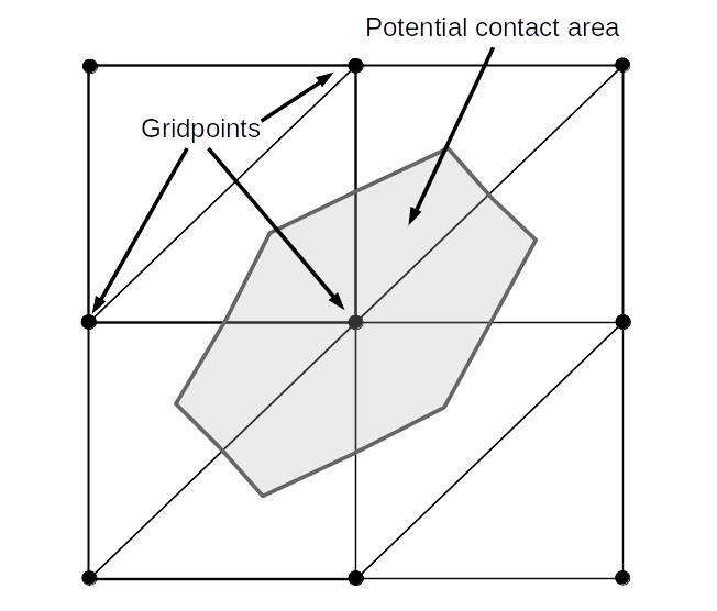
Figure 1: Gridpoints, zone joint facets and potential contact area associated with a gridpoint in 3D. This view is looking down on the joint.

The potential contact area in 2D is shown in the figure below. This area extends half way between vertices/gridpoints on either side of the vertex/gridpoint at the center. As with 3D, each gridpoint corresponds uniquely to one wall vertex.

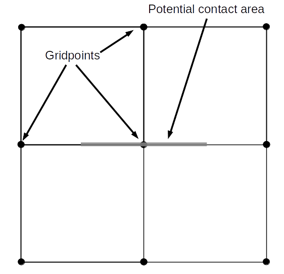
Figure 2: Gridpoints, zone joint facets and potential contact area associated with a gridpoint in 2D.

Contacts exist between the wall vertices on one side of the joint and wall facets on the other side. Call the joint surface in the 3D figure above side A, or the top of the joint in the 2D figure. Suppose that joint surface B, corresponding to zone faces on the opposing side of the joint, is coincident with joint surface A. The shaded area of side A is broken into {line segments in 2D; triangles in 3D} that are clipped against the overlapping facets of side B. The clipping operation allows one to determine: 1) the facets on B associated with this contact, 2) the area of contact, and 3) vertex weights for side B, to compute relative velocities and to distribute forces to the gridpoints on side B. The weights are computed via barycentric interpolation/extrapolation, as outlined in this section, in 3D. In 2D the same barycentric notion applies but with simpler geometry. If the wall facets and vertices between sides A and B are identical then the barycentric strategy results in one vertex on side B with non-zero weight, i.e., the vertex/gridpoint directly opposing the vertex/gridpoint on side A. The wall facets and vertices do not need to mirror one another across the joint surface for the clipping/barycentric scheme to produce sensible contact areas and weights. For each joint, the side with the most wall vertices is used as side A above.

Complex intersections between joint surfaces are accommodated by splitting the edge connected surfaces on each side of the joint into separate walls. The figure below depicts one side of a joint that is intersected by a joint in the out-of-plane direction along the diagonal in 3D. The darker triangular facets on the upper left are grouped into one wall, while the lighter triangular facets on the lower right are grouped into a separate wall. These walls have distinct vertices and facets. As mentioned above, since all separations must happen prior to zone joint creation, the gridpoints are also unique on each side of the intersection. Two potential contact areas result that are independent of one another, resulting in potentially two independent contacts on either side of the intersection.

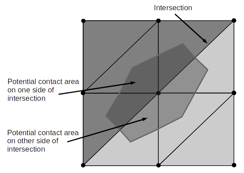
Figure 3: Joint surface intersected by another joint in the out-of-plane direction.

As alluded to above, the creation of zone joints is a four stage process: 1) configure the engine for zone joitns, 2) separation of all internal discontinuities to produce distinct sets of zone joint faces, 3) wrapping the zone joint faces with wall vertices/facets and 4) resolving contacts between wall vertices and wall facets on opposing sides of coincident joint surfaces.