Cylindrical Hole in an Infinite Mohr-Coulomb Medium

Problem Statement

Note

To view this project in 3DEC, use the menu command Help ► Examples…. The main data files used are shown at the end of this example. All data files are found in the project.

This problem concerns determination of stresses and displacements around a cylindrical hole in an infinite elasto-plastic medium subjected to a compressive, isotropic far-field stress. The objective of this problem is to test the plasticity calculations in 3DEC. The medium is assumed to be linearly elastic, perfectly plastic. The Mohr-Coulomb criterion is used as the plastic limit; the material deforms plastically according to the associated flow rule (i.e., the dilation angle is equal to the friction angle).

The material is assigned the following properties:

density (\(\rho\)): 2600 kg/m³

shear modulus (\(G\)): 2.8 GPa

bulk modulus (\(K\)): 3.9 GPa

cohesion (\(c\)): 3.45 MPa

friction angle (\(\phi\)): 30°

dilation angle (\(\psi\)): 30°

An isotropic far-field stress is equal to 30 MPa. The radius of the hole is 1 m, and is assumed to be small compared to the length of the cylinder. (This permits the use of the plane-strain solution for comparison.)

Analytic Solution

The radius of the plastic zone, \(R_o\), around a circular cylindrical hole in an infinite Mohr-Coulomb material (Figure 1) is given by the analytical solution derived by Salençon (1969):

\[R_o = a\ \left ( \thinspace {2 \over {K_p + 1}}\ {P_o + {q \over {K_p - 1}} \over {P_i + {q \over {K_p - 1}}}}\thinspace \right )^{1/(K_p - 1)}\]

where:

\(a\) = radius of hole;

\(K_p\) = \((1 + \sin \phi)/ (1 -\sin \phi)\);

\(q\) = \(2c \tan (45 + \phi /2)\);

\(P_o\) = initial in-situ stress; and

\(P_i\) = internal pressure.

According to the solution, the radial stress at the elastic/plastic interface is

\[\sigma_{re} = {1 \over {K_p + 1}}\ (2 P_o - q)\]

The stresses in the plastic zone are:

\[\sigma_r = -{q \over {K_p - 1}} + \left(P_i + {q \over {K_p - 1}}\right) \cdot \left({r \over {a}}\right)^{K_p - 1}\]

\[\sigma_\theta = -{q \over {K_p - 1}} + K_p \left(P_i + {q \over {K_p - 1}}\right) \cdot \left({r \over {a}}\right)^{K_p - 1}\]

where \(r\) is the distance to the center of the hole; and the stresses in the elastic zone are:

\[\sigma_r = P_o - (P_o - \sigma_{re})\ \cdot\ \left({R_o \over {r}}\right)^2\]

\[\sigma_\theta = P_o + (P_o - \sigma_{re})\ \cdot\ \left({R_o \over {r}}\right)^2\]

The displacements in the elastic zone are

\[u_r = \left[P_o - \left({2 P_o - q \over {K_p + 1}} \right) \right]\ \left({R_o \over {2G}} \right)\ \left( {R_o \over {r}}\right)\]

and in the plastic region are:

\[u_r = {r \over {2G}} \chi\]

\[\chi = (2 \nu - 1)\ \left(P_o + {q \over {K_p -1}}\right)\]

\[+ {(1 - \nu) (K^2_p - 1) \over {K_p + K_{ps}}} \left(P_i + {q \over {K_p - 1}}\right)\ \left({R_o \over {a}}\right)^{(K_p - 1)}\ \left({R_o \over {r}}\right)^ {(K_{ps} + 1)}\]

\[+ \left[(1 - \nu)\ {{K_p K_{ps} + 1} \over {K_p + K_{ps}}} - \nu\right]\ \left(P_i + {q \over {K_p - 1}}\right)\ \left({r \over {a}}\right)^{(K_p - 1)}\]

where:

\(K_{ps}\) = \((1 + \sin \psi)/(1 − \sin \psi)\) ;

\(\psi\) = dilation angle; and

\(\nu\) = Poisson’s ratio.

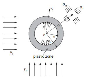
Figure 1: Cylindrical hole in an infinite Mohr-Coulomb medium.

3DEC Model

The geometry of the 3DEC model used for this analysis is shown in Figure 2. The model is constrained in the direction of the \(x\)-axis, so that it can only move in the \(yz\)-plane (plane-strain condition). The model consists of 900 joined blocks in a radial pattern. The boundary was selected at 10 m (i.e., five hole-diameters) from the hole center. The problem was solved using three different types of zoning. In the first case, a mixed-discretization (hex) zoning was used to discretize 900 blocks into 9000 zones. (An accurate solution of elasto-plastic problems requires finer zoning than is needed for the simulation of linearly elastic problems.) Figure 3 shows the geometry of blocks and zones for this case. (There is one hex zone — i.e., two sets of 5 overlapping tetrahedra per block.) In the second case, 900 blocks were discretized into 50,900 “regular” tetrahedral zones. The geometry of the zones on one side of the model is shown in Figure 4. In all cases, the blocks were joined (i.e., the discontinuities between blocks have no effect on deformation of the model). In the third case, 900 blocks were discretized into 1096 higher-order zones. The geometry of the zones on one side of the model is shown in Figure 5.

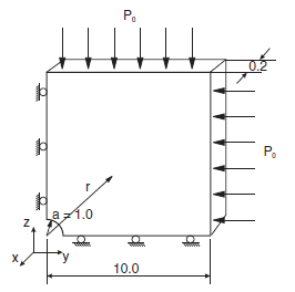
Figure 2: 3DEC model geometry used for analysis of cylindrical hole in a Mohr-Coulomb medium.

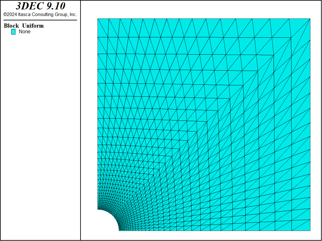
Figure 3: Blocks and “hex” zones in 3DEC model.

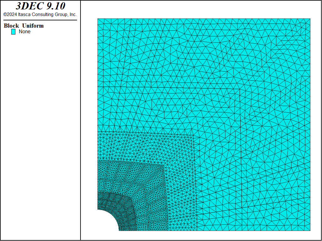
Figure 4: Tetrahedral zones in 3DEC model.

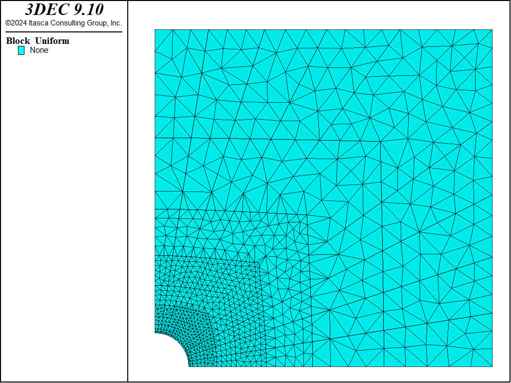
Figure 5: High-order tetrahedral zones in 3DEC model.

Results and Discussion

Because the problem is axisymmetric, all results are presented as a function of the distance from the center of the opening. Figures 6 and 7 compare 3DEC results using hex zoning with the analytical solution. (The radial displacements are compared in Figure 6; the radial and tangential stresses are compared in Figure 7.) The plots show excellent agreement between the two results. Note the 3DEC stresses plotted in Figure 7 are not tetrahedral zone stresses, but stresses obtained by averaging the tetrahedral stresses on the level of the hex zones. (Even in the case of hex zoning, stresses in 3DEC are stored in tetrahedral zones. Quad-zone stresses (i.e., average stresses on the level of a hex zone) are calculated during the calculation of velocities and stress increments only.) A FISH function was used to calculate the average stresses (see “mchole.fis”) .

Results obtained with 3DEC using tetrahedral zoning are compared with the analytical solution in Figures 8 and 9. Agreement between displacements in Figure 8 is excellent. The numerical results deviate from the analytical solution in the vicinity of the far-field boundaries only. (The error is a consequence of the finite size of the numerical model and approximate boundary conditions.) The results for stresses in Figure 9 show large numerical dispersion in the plastic region. Such a result is expected behavior for tetrahedral zones (or triangular zones in 2D) with linear approximation of displacements (or constant approximation of strains and stresses). Mixed discretization, the methodology which is used to improve performance of tetrahedral (or triangular) zones in elastoplastic calculations, is implemented with hex zoning in 3DEC. Results obtained with 3DEC using the high-order tetrahedral zones are compared with the analytical solution in Figures 10 and 11. Agreements between displacements in Figure 10 is excellent. The results for the stresses in Figure 11 are almost as good as the results obtained using the mixed discretization. These results were obtained using only a fraction of the elements needed for the other methods. The different zoning approaches have the following disadvantages:

1. Quad zoning cannot be used for discretization of arbitrarily shaped blocks.

2. Stress fields calculated with tetrahedral zones for elasto-plastic problems are not smooth.

Figure 6: Comparison of radial displacements as a function of radius.

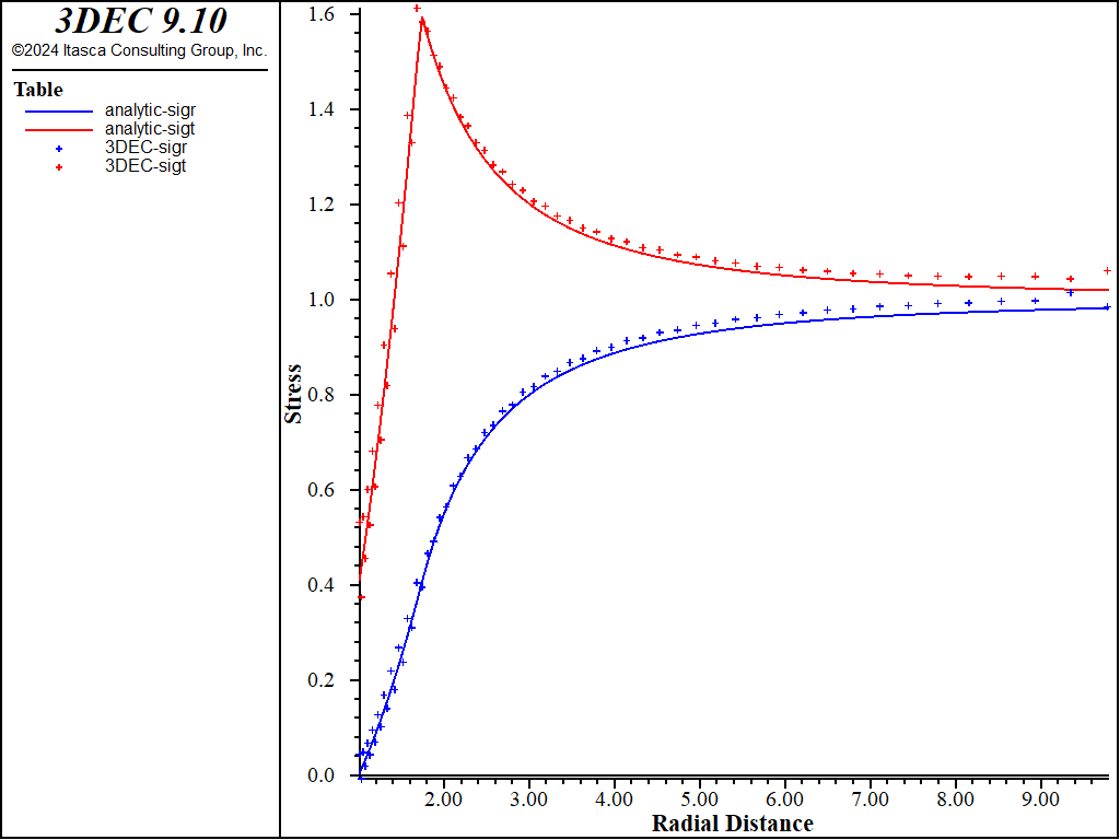
Figure 7: Comparison of radial and tangential normal stresses as a function of radius.

Figure 8: Comparison of radial displacements as a function of radius, using tetrahedral zones.

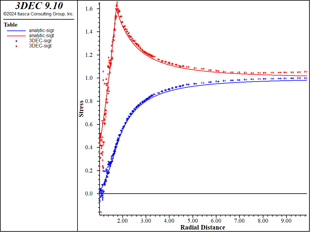
Figure 9: Comparison of radial and tangential normal stresses as a function of radius, using tetrahedral zones.

Figure 10: Comparison of radial displacements as function of radius, using high-order tetrahedral zones.

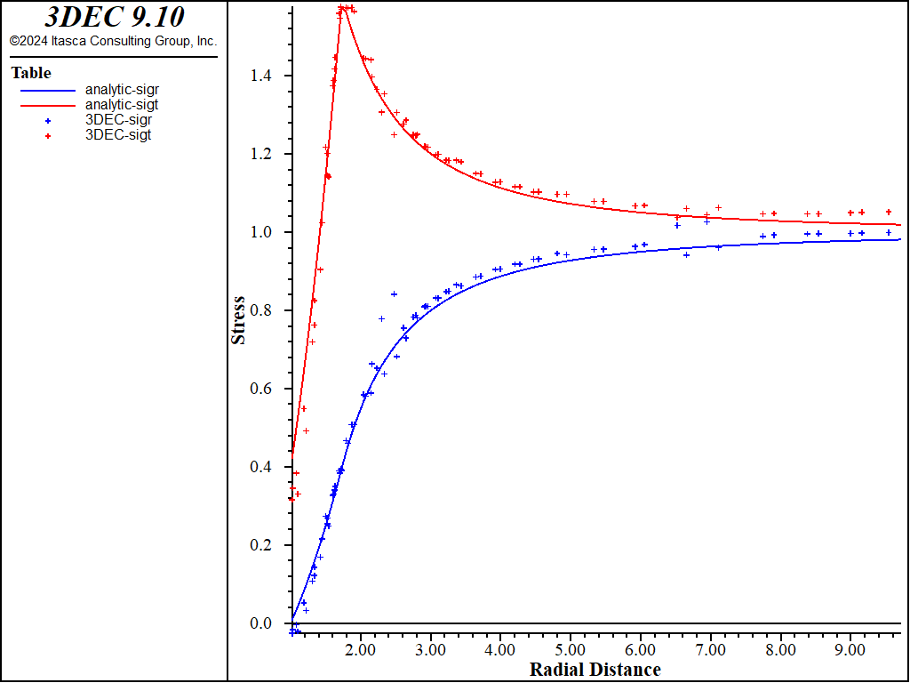
Figure 11: Comparison of radial and tangential normal stresses as a function of radius, using high-order tetrahedral zones

Reference

Salençon, J. “Contraction Quas-Statique D’une Cauite a Symetric Spherique Ou Cylindrique Dans Un Milieu Elastoplastique,” Annales Des Ports Et Chaussees, Vol. 4, pp. 231-236 (1969).

Data Files

mchole-hex.dat

;==========================================================================
; verification test -- 3dec modeling cylindrical hole in an infinite,
;                      isotropic, homogeneous, Mohr-Coulomb medium
; quadrilateral zoning
; Mohr-Coulomb blocks
;
;==========================================================================
model new

model large-strain off 

block create tunnel dip 0 dip-direction 0 radius 1 length 0 0.2 ...
                    blocks-axial 1 blocks-radial 30 blocks-tangential 15 ...
                    boundary 9 radius-ratio 1.07
block delete range cylinder end-1 0 0 0 end-2 0 1 0 radius 0 1
block delete range plane dip 0 dip-direction 0 below
block delete range plane dip 90 dip-direction 90 below

block join on
;
; --- zoning of blocks ---
;
block zone generate hexahedra divisions 1 1 1
;
; --- material properties ---
;
block zone cmodel assign mohr-coulomb
block zone property bulk 3.9e9 shear 2.8e9 density 2600 
block zone property cohesion 3.45e6 tension 1e7 friction 30 dilation 30 
;
; --- boundary conditions ---
block face apply stress -30e6 -30e6 -30e6 0 0 0 range position-x 10
block face apply stress -30e6 -30e6 -30e6 0 0 0 range position-z 10
block gridpoint apply velocity-x 0 range position-x 0
block gridpoint apply velocity-y 0 range position-y 0
block gridpoint apply velocity-y 0 range position-y 0.2
block gridpoint apply velocity-z 0 range position-z 0
;
; --- initial conditions ---
;
block insitu stress -30e6 -30e6 -30e6 0 0 0
;
model history mechanical unbalanced-maximum
;
; if there are no joints, local damping should be used
block mechanical damping local 0.8
model solve

program call 'mchole.fis'
model save 'mchole-hex'
;
program return

mchole-tet.dat

;==========================================================================
; verification test -- 3dec modeling cylindrical hole in an infinite,
;                      isotropic, homogeneous, Mohr-Coulomb medium
; tetrahedral zoning
; Mohr-Coulomb blocks
;
;==========================================================================
model new

model large-strain off

model random 10000
block create tunnel dip 0 dip-direction 0 radius 1 length 0 0.2 ...
                    blocks-axial 1 blocks-radial 10 blocks-tangential 5 ...
                    boundary 9 radius-ratio 1.4
block delete range cylinder end-1 0 0 0 end-2 0 1 0 radius 0 1
block delete range plane dip 0 dip-direction 0 below
block delete range plane dip 90 dip-direction 90 below

block join on
;
; --- zoning of blocks ---
;
block zone generate edgelength 0.05 range position-x 0 1.7 position-z 0 1.7
block zone generate edgelength 0.08 range position-x 0 2.9 position-z 0 2.9
block zone generate edgelength 0.15 range position-x 0 5.3 position-z 0 5.3
block zone generate edgelength 0.30
;
; --- material properties ---
;
block zone cmodel assign mohr-coulomb
block zone property bulk 3.9e9 shear 2.8e9 density 2600
block zone property cohesion 3.45e6 tension 1e7 friction 30 dilation 30
;
; --- boundary conditions ---
block face apply stress -30e6 -30e6 -30e6 0 0 0 range position-x 10
block face apply stress -30e6 -30e6 -30e6 0 0 0 range position-z 10
block gridpoint apply velocity-x 0 range position-x 0
block gridpoint apply velocity-y 0 range position-y 0
block gridpoint apply velocity-y 0 range position-y 0.2
block gridpoint apply velocity-z 0 range position-z 0
;
; --- initial conditions ---
;
block insitu stress -30e6 -30e6 -30e6 0 0 0
;
model history mechanical unbalanced-maximum

; if there are no joints, local damping should be used
block mechanical damping local 0.8
model solve

program call 'mchole.fis'
model save 'mchole-tet'
;
program return

mchole-ho.dat

;==========================================================================
; verification test -- 3dec modeling cylindrical hole in an infinite,
;                      isotropic, homogeneous, Mohr-Coulomb medium
; High order tetrahedral zoning
; Mohr-Coulomb blocks
;
;==========================================================================
model new

model large-strain off

model configure highorder

block create tunnel dip 0 dip-direction 0 radius 1 length 0 0.2 ...
                    blocks-axial 1 blocks-radial 10 blocks-tangential 5 ...
                    boundary 9 radius-ratio 1.4
block delete range cylinder end-1 0 0 0 end-2 0 1 0 radius 0 1
block delete range plane dip 0 dip-direction 0 below
block delete range plane dip 90 dip-direction 90 below

block join on
;
; --- zoning of blocks ---
;
block zone generate edgelength 0.3 range position-x 0.0 1.7 position-z 0.0 1.7
block zone generate edgelength 0.6 range position-x 0.0 2.9 position-z 0.0 2.9
block zone generate edgelength 0.8 range position-x 0.0 5.3 position-z 0.0 5.3
block zone generate edgelength 1
block zone generate high-order-tetra
;
; --- material properties ---
;
block zone cmodel assign mohr-coulomb
block zone property bulk 3.9e9 shear 2.8e9 density 2600 
block zone property cohesion 3.45e6 tension 1e7 friction 30 dilation 30 
;
; --- boundary conditions ---
block face apply stress -30e6 -30e6 -30e6 0 0 0 range position-x 10
block face apply stress -30e6 -30e6 -30e6 0 0 0 range position-z 10
block gridpoint apply velocity-x 0 range position-x 0
block gridpoint apply velocity-y 0 range position-y 0
block gridpoint apply velocity-y 0 range position-y 0.2
block gridpoint apply velocity-z 0 range position-z 0
;
; --- initial conditions ---
;
block insitu stress -30e6 -30e6 -30e6 0 0 0
;
model history mechanical unbalanced-maximum
;
; if there are no joints, local damping should be used
block mechanical damping local 0.8
model solve
program call 'mchole.fis'

model save 'mchole-ho'
;
program return

mchole-nmd.dat

;==========================================================================
; verification test -- 3dec modeling cylindrical hole in an infinite,
;                      isotropic, homogeneous, Mohr-Coulomb medium
; Nodal Mixed Discretization zoning
; Mohr-Coulomb blocks
;
;==========================================================================
model new

model large-strain off

block create tunnel dip 0 dip-direction 0 radius 1 length 0 0.2 ...
                    blocks-axial 1 blocks-radial 10 blocks-tangential 5 ...
                    boundary 9 radius-ratio 1.4
block delete range cylinder end-1 0 0 0 end-2 0 1 0 radius 0 1
block delete range plane dip 0 dip-direction 0 below
block delete range plane dip 90 dip-direction 90 below

block join on
;
; --- zoning of blocks ---
;
block zone generate edgelength 0.1 range position-x 0 1.7 position-z 0 1.7
block zone generate edgelength 0.16 range position-x 0 2.9 position-z 0 2.9
block zone generate edgelength 0.3 range position-x 0 5.3 position-z 0 5.3
block zone generate edgelength 0.6
;
; --- material properties ---
;
block zone cmodel assign mohr-coulomb
block zone property bulk 3.9e9 shear 2.8e9 density 2600 
block zone property cohesion 3.45e6 tension 1e7 friction 30 dilation 30 

block zone nodal-mixed-discretization on
;
; --- boundary conditions ---
block face apply stress -30e6 -30e6 -30e6 0 0 0 range position-x 10
block face apply stress -30e6 -30e6 -30e6 0 0 0 range position-z 10
block gridpoint apply velocity-x 0 range position-x 0
block gridpoint apply velocity-y 0 range position-y 0
block gridpoint apply velocity-y 0 range position-y 0.2
block gridpoint apply velocity-z 0 range position-z 0
;
; --- initial conditions ---
;
block insitu stress -30e6 -30e6 -30e6 0 0 0
;
model history mechanical unbalanced-maximum

; if there are no joints, local damping should be used
block mechanical damping local 0.8
model solve

program call 'mchole.fis'

model save 'mchole-nmd'

program return

mchole.fis

;---------------------------------------------------------------------
;    exact and numerical solution processing for salencon problem
;
;    nastr, stores in
;    Table 1: analytical values rad/a -sigr/p0
;    Table 2: analytical values rad/a -sigt/p0
;    Table 3: numerical values rad/a -sigr/p0
;             at zone centroid closest to x axis
;    Table 4: numerical values rad/a -sigt/p0
;             at zone centroid closest to x axis
;
;    and calculates in whole grid
;    errsr  : average %error in -sigr/p0
;    errst  : average %error in -sigt/p0
;
;    nadis, stores in
;    Table 5: analytical values of rad/a -ur/a
;    Table 6: numerical  values of rad/a -ur/a at grid points on x axis
;
;    and calculates in whole grid
;    errd   : average %error in modulus of displacement
;---------------------------------------------------------------------
fish automatic-create off
;
;--- access property (cohesion, friction) and grid information ---
fish define const
  global po = 30.0e6 ; far-field stress
  global kp
  global kpm1
  global cqk
  global sre
  global ro
  global kpsp1
  global xi1
  global xi2
  global xi3
  global coe
  
  ; material properties
  local cco = 3.45e6
  local cfi = 30.0*math.degrad
  local cdi = 30.0*math.degrad
  local bm    = 3.3e9
  local sm    = 2.8e9
  local nu    = (3.*bm-2.*sm)/(6.*bm+2.*sm)
  
  kp    = (1.+math.sin(cfi))/(1.-math.sin(cfi))
  kpm1  = kp - 1
  local cq    = 2.*cco*math.cos(cfi)/((1.0-math.sin(cfi))*po)
  cqk   = cq/(kp-1.)
  sre   = (2.-cq)/(kp+1.)
  ro    = (2.*(1.+cqk)/((kp+1.)*cqk))^(1./kpm1)
  local kps   = (1.+math.sin(cdi))/(1.-math.sin(cdi))
  kpsp1 = kps+1
  xi1   = (2.*nu-1.)*(1.+cqk)
  xi2   = ((1.-nu)*(kp^2-1.)/(kp+kps))*cqk*ro^kpm1
  xi3   = ((1.-nu)*(kp*kps+1)/(kp+kps)-nu)*cqk
  coe   =  po/(2.*sm)
end
; =================================================
; Stresses
; =================================================
fish define nastr
    local numrad = 0
    local tab1  = table.get(1)
    local tab2  = table.get(2)
    local tab3  = table.get(3)
    local tab4  = table.get(4)
    table.label(tab1) = 'analytic-sigr'
    table.label(tab2) = 'analytic-sigt'
    table.label(tab3) = '3DEC-sigr'
    table.label(tab4) = '3DEC-sigt'
    global errsr
    global errst
    errsr = 0.0
    errst = 0.0
	
    loop foreach local iz_ block.zone.list
         local mark = 0
         local igp
         loop igp (1,4)
              local gpind = block.zone.gp(iz_,igp)
              if block.gp.pos.z(gpind) < 0.001 then
                 mark = mark + 1
              end_if
         end_loop
         local rad = math.sqrt(block.zone.pos.x(iz_)^2 + ...
                     block.zone.pos.z(iz_)^2)
         local theta_ = math.atan2(block.zone.pos.z(iz_),block.zone.pos.x(iz_))
         if rad < ro then
            local aux1  = rad^kpm1
            local sigre = -cqk*(1.-aux1)
            local sigte = -cqk*(1.-kp*aux1)
         else
            aux1  = (1.-sre)*(ro/rad)^2
            sigre = 1. - aux1
            sigte = 1. + aux1
         end_if
         local stemp1 = 0.5*(block.zone.stress.xx(iz_) + ...
                        block.zone.stress.zz(iz_))
         local stemp2 = 0.5*(block.zone.stress.xx(iz_) - ...
                        block.zone.stress.zz(iz_))
         local stemp3 = block.zone.stress.xz(iz_)*math.sin(2.0*theta_)
         local sigr = -(stemp1 + stemp2*math.cos(2.0*theta_)+stemp3)/po
         local sigt = -(stemp1 - stemp2*math.cos(2.0*theta_)-stemp3)/po
         if mark > 2
            numrad = numrad + 1
            table(tab1,rad) = sigre
            table(tab2,rad) = sigte
            table(tab3,rad) = sigr
            table(tab4,rad) = sigt
         end_if
         local err = math.abs(sigr - sigre)
         errsr = errsr + err
         err = math.abs(sigt - sigte)
         errst = errst + err
    end_loop
    errsr = errsr * 100. / block.zone.num
    errst = errst * 100. / block.zone.num
end
; =================================================
; Displacements
; =================================================
fish define nadis
    global numrad
    numrad = 0
    local tab5  = table.get(5)
    local tab6  = table.get(6)
    table.label(tab5) = 'analytic-ur'
    table.label(tab6) = '3DEC-ur'
    local rad = 1.
    local dism = coe*rad*(xi1+xi2*(ro/rad)^kpsp1+xi3*rad^kpm1)
    global errd
    errd = 0.0
    
    loop foreach local igp_ block.gp.list
         local mark = 0
         if block.gp.pos.z(igp_) < 0.001 then
            if block.gp.pos.y(igp_) < 0.001 then
              mark = 1
            end_if
         end_if
         rad = math.sqrt(block.gp.pos.x(igp_)^2 + block.gp.pos.z(igp_)^2)
         if rad < ro then
            local dise = coe*rad*(xi1+xi2*(ro/rad)^kpsp1+xi3*rad^kpm1)
         else
            dise = coe*(1.-sre)*ro^2/rad
         end_if
         local dis = math.sqrt(block.gp.disp.x(igp_)^2 + ...
                     block.gp.disp.z(igp_)^2)
         local err = math.abs(dis - dise)
         errd = errd + err
         if mark = 1 then
            numrad = numrad + 1
            table(tab5,rad) = 100*dise
            table(tab6,rad) = 100*dis
         end_if
    end_loop
    errd = errd * 100. / (dism * block.zone.num)
end
;
[const]
[nastr]
[nadis]
;
fish list [numrad]
fish list [errsr]
fish list [errst]
fish list [errd]
fish automatic-create on
; eof

Endnote

[1]

This example is listed under the present document title in the i Examples dialog use the menu command Help -> Examples… to access.