FLAC3D Theory and Background • Fluid-Mechanical Interaction

One-Dimensional Consolidation (FLAC2D)

Note

The project file for this example is available to be viewed/run in FLAC2D. The project’s main data files are shown at the end of this example.

A saturated layer of soil of thickness \(H\) = 20 m (shown in Figure 1) and large horizontal extent rests on a rigid impervious base. A constant surface load, \(p_z\) = 10⁵ Pa, is applied on the layer under undrained conditions. The soil matrix is homogeneous and behaves elastically; the isotropic Darcy’s transport law applies. The applied pressure is initially carried by the fluid, but as time goes on the fluid drains through the layer surface, transferring the load to the soil matrix. The solution to this one-dimensional consolidation problem may be expressed in the framework of Biot theory (see Detournay and Cheng 1993).

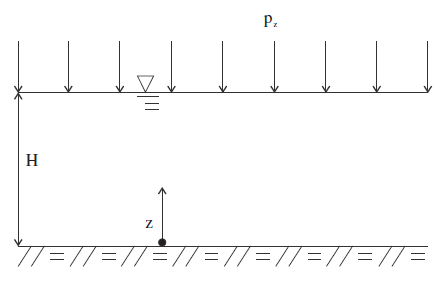
Figure 1: One-dimensional consolidation.

The diffusion equation for the pore pressure, \(p\), has the form

(1)\[{{\partial p}\over{\partial t}} - c {{{\partial}^2p}\over{\partial y^2}} = - {{\alpha}\over{\alpha_1 S}} {{d {\sigma}_{yy}}\over{dt}}\]

where:	\(c\)	=	\(k/S\);
	\(S\)	=	\(1/M + \alpha^2/\alpha_1\) = the storage coefficient;
	\(\alpha_1\)	=	\(K + 4G/3\);
	\(M\)	=	the Biot modulus; and
	\(\alpha\)	=	the Biot coefficient.

The boundary conditions are \(\sigma_{yy}\) = \(-p_y H(t)\) and \(p\) = 0 at \(y\) = H (\(H(t)\) is the step function), and \(u_y\) = 0 and \({{\partial p}\over{\partial y}}\) = 0 at \(y\) = 0.

Because the stress is constant, Equation (1) reduces to

(2)\[{{\partial p}\over{\partial t}} - c {{{\partial}^2p}\over{\partial y^2}} = 0\]

with boundary conditions \(p\) = 0 at \(y = H\), and \({{\partial p}\over{\partial y}}\) = 0 at \(y\) = 0.

The initial value, \(p_0\), for the pore pressure induced from loading of the layer may be derived from the fluid constitutive law (\(p = M(\zeta - \alpha {\epsilon}_{yy})\)) by considering undrained conditions (\(\zeta\) = 0) and using the one-dimensional mechanical constitutive law (\({\sigma}_{yy} = \alpha_1 {\epsilon}_{yy} - \alpha p\)) to express strain in terms of stresses. It is given by

(3)\[p_0 = {{\alpha}\over{\alpha_1}} {{1}\over{S}} {p_y}\]

The solution for the pore pressure is

(4)\[\hat{p} = 2{{p_0}\over{p_y}} \sum_{m=0}^{\infty} {{\sin (a_m \hat{y})}\over{a_m}} e^{-a_m^2 \hat{t}}\]

where:	\(\hat{p}\)	=	\(p/p_y\);
	\(a_m\)	=	\((2 m +1)\pi/2\);
	\(\hat{y}\)	=	\((H-z)/H\); and
	\(\hat{t}\)	=	\(ct/H^2\).

The vertical displacement, \(u_y\), is found by considering the equilibrium equation \(\partial {\sigma}_{yy} / \partial y\) = 0 together with the mechanical constitutive equation \({\sigma}_{yy} = \alpha_1 {\epsilon}_{yy} - \alpha p\). By expressing \({\epsilon}_{yy}\) as \(\partial u_y / \partial y\), we obtain upon integration, taking Equation (4) and the boundary conditions into account,

(5)\[{\hat{u}}_y = 2 \alpha {{p_0}\over{p_y}} \left [ \sum_{m = 0}^{\infty} {{\cos (a_m \hat{y})}\over{a_m^2}} e^{-a_m^2 \hat{t}} \right ] + {\hat{y} - 1}\]

here \({\hat{u}}_y\) is defined as \({\hat{u}}_y = {{\alpha_1 u_y}\over{H p_y}}\).

The following properties are prescribed for this example:

dry bulk modulus, \(K\)	5 × 108 Pa
dry shear modulus, \(G\)	2 × 108 Pa
Biot modulus, \(M\)	4 × 109 Pa
Biot coefficient, \(\alpha\)	1.0
permeability, \(k\)	10-10 m2/Pa-sec

The FLAC2D model grid for this problem is a column of 20 zones of unit dimensions lined up along the \(y\)-axis. (See Figure 2.) The base of the column is fixed, and lateral displacements are restricted in the \(x\) direction. A mechanical pressure, \(p_y\), is applied at the top of the column.

At first, flow is prevented and the model is stepped to equilibrium to establish the initial undrained conditions. At the end of this stage, the stress \({\sigma}_{yy}\) has the value \(-p_y\), in equilibrium with the applied pressure, and the pore pressure has the initial undrained value \(p_0 = \alpha p_y/\alpha_1 S\) (see Figure 3). Drainage is then allowed by setting the pore pressure to zero at the top of the column. The FLAC2D model is cycled to a flow time of 5000 seconds, which is approximately the magnitude of the characteristic time, \(t_c = H^2/c\), for this problem.

The analytical solution for the pore pressure, \(\hat{p}\), and vertical displacement, \({\hat{u}}_y\), at the column mid-height are evaluated using FISH functions, and compared to the numerical solution as time proceeds. The results are plotted versus fluid-flow time in Figure 3 and Figure 4. The transfer of pore pressure to effective stress is illustrated in Figure 5, where the evolution of normalized total stress, \(-{\sigma}_{yy} / p_y\), effective stress, \(-({\sigma}_{yy} + p) / p_y\), and pore pressure, \(p / p_y\), with fluid-flow time are presented. The FLAC2D data file is listed in “1DConsolidation-Coupled.dat”.

break

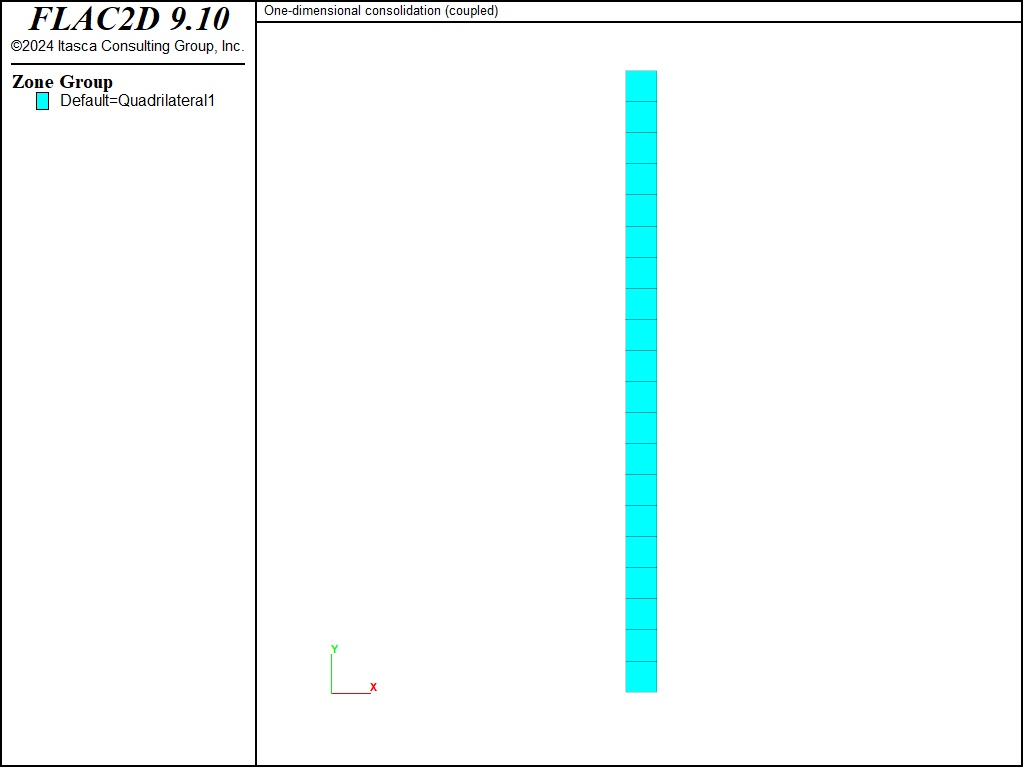
Figure 2: FLAC2D grid for one-dimensional consolidation.

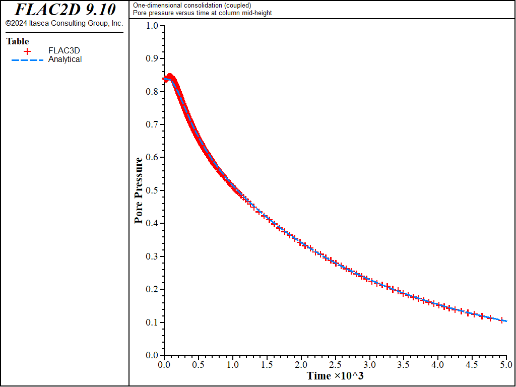
Figure 3: Comparison between analytical and numerical values of pore pressure in a 1D consolidation test — \(M\) = 4 × 10⁹ Pa.

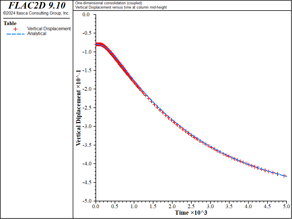
Figure 4: Comparison between analytical and numerical values for vertical displacement in a 1D consolidation test — \(M\) = 4 × 10⁹ Pa.

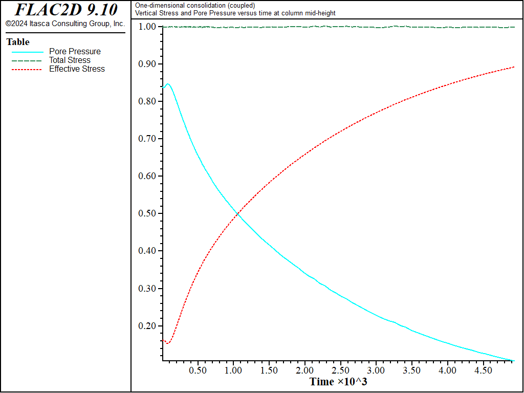
Figure 5: Evolution of pore pressure, total and effective stresses in a 1D consolidation test — \(M\) = 4 × 10⁹ Pa.

Note that as the stiffness ratio \(R_k = \alpha^2 M/(K + 4G/3)\) increases, the number of zones should increase to keep the error small. This effect is caused by the numerical technique used to evaluate pore-pressure changes caused by volumetric strain in model configure fluid-flow. Also, as the ratio \(R_k\) increases, the timestep will decrease. However, to keep the error small and the timestep sufficiently large without significantly affecting the solution, it is acceptable to limit the value of Biot modulus (or \(K_f\)) used in the simulation to a value of approximately twenty times \((K + 4G/3)/{\alpha^2}\) (see the fifth item in Solving Flow-Only and Coupled-Flow Problems, and the zone fluid modulus-automatic command). To demonstrate the validity of this numerical approach, the analytical solutions for pore pressure and displacement corresponding to \(M\) = 1.5 × 10¹⁰ (\(R_k \simeq\) 20) and \(M\) = 1.5 × 10¹⁵ (\(R_k \simeq\) 20 × 10⁵) are compared in Figure 6 and Figure 7. As seen in those plots, the responses are indeed similar (maximum relative error less than 5%).

break

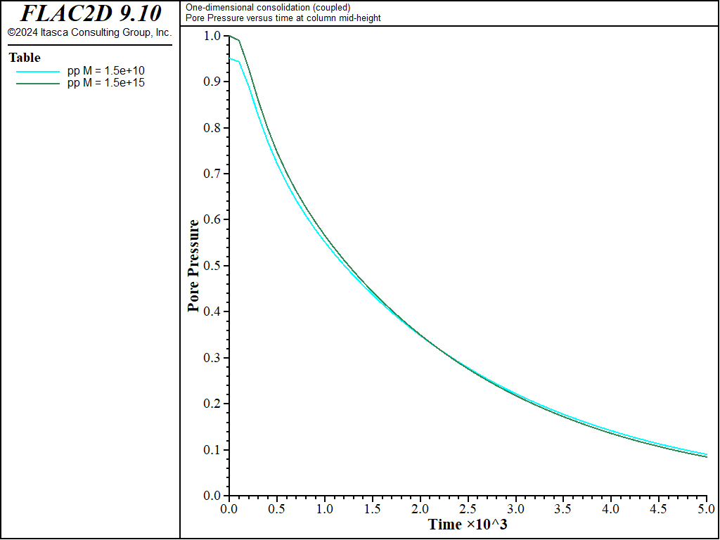
Figure 6: Comparison between analytical pore-pressure solutions for two large values of M in a 1D consolidation test.

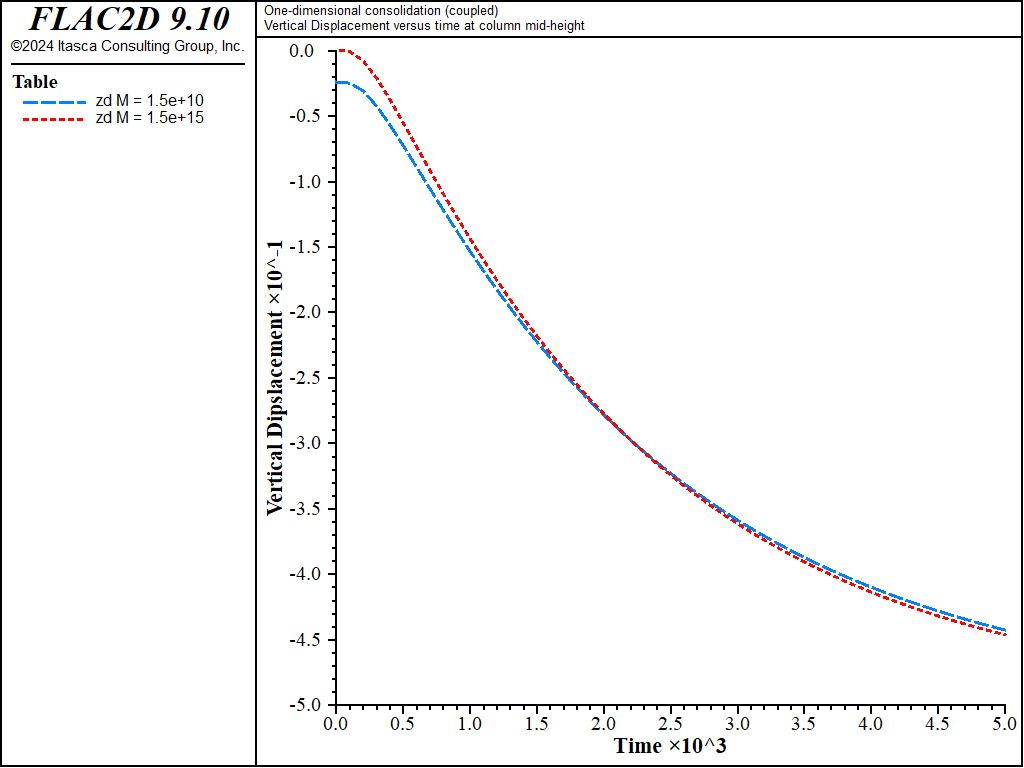
Figure 7: Comparison between analytical vertical displacement solutions for two large values of M in a 1D consolidation test.

For values of the stiffness ratio, \(R_k\), much larger than 20, the convergence of the basic algorithm for coupled fluid flow will be very slow (i.e., numerous mechanical steps will be necessary to bring the system to mechanical equilibrium after each flow step). This is illustrated by repeating the couple test with Biot modulus \(M\) = 4 × 10¹⁰ Pa (10 times larger than in the former numerical calculation, see 1DConsolidation-Coupled10M.dat). In the former calculation with \(M\) = 4 × 10⁹ Pa (\(R_k\) = 5.2), the coupled flow calculation ran in approximately 4 seconds (on a 1.6 GHz i7 computer). For the calculation with \(M\) = 4 × 10¹⁰ Pa (\(R_k\) = 52), the calculation time is approximately 40 seconds (ten times slower). The comparison of the pore pressure and displacement history results to the analytical solutions for \(M\) = 4 × 10¹⁰ Pa are shown in Figure 8 and Figure 9, respectively. The maximum relative error is less than 4%.

break

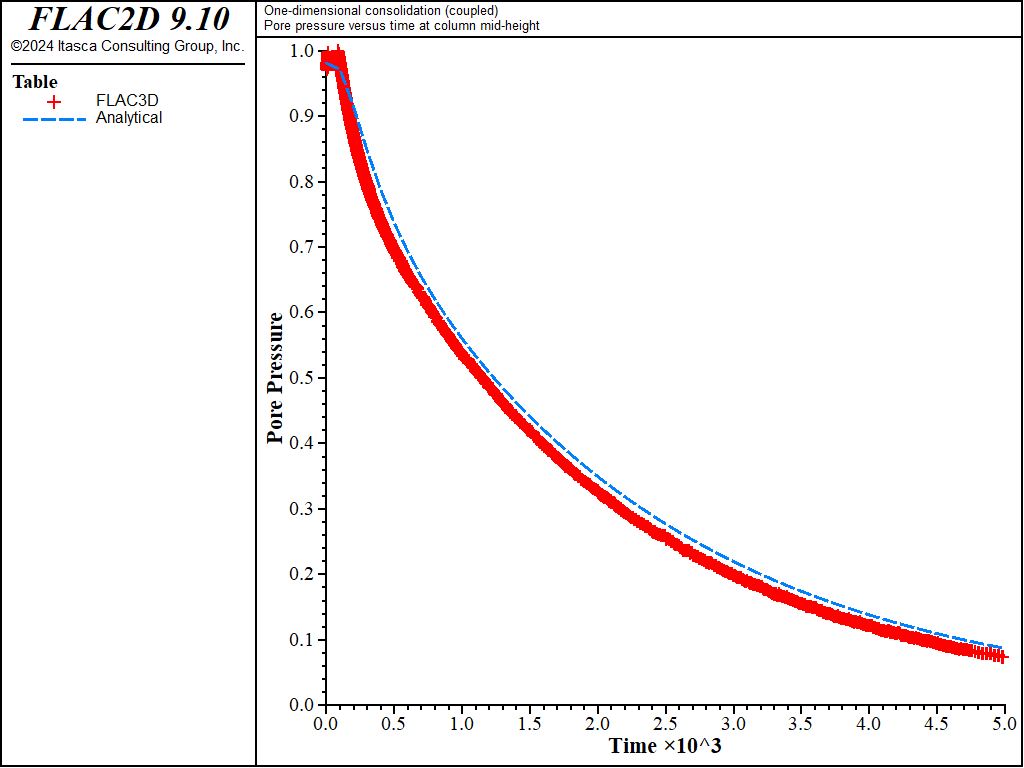
Figure 8: Comparison between analytical and numerical values of pore pressure in a 1D consolidation test - \(M\) = 4 × 10¹⁰ Pa.

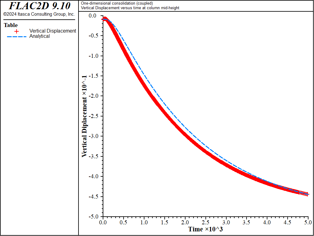
Figure 9: Comparison between analytical and numerical values for vertical displacement in a 1D consolidation test - \(M\) = 4 × 10¹⁰ Pa.

The solution time can be reduced by using the uncoupling technique described in Stiffness Ratio (the applicability of the uncoupling technique to this problem follows from the irrational character of the solution). In this test (1DConsolidation-Uncoupled.dat), the numerical simulation is repeated for a Biot modulus of 4 × 10¹⁰ Pa using the uncoupling technique. In this test, the initial undrained conditions are obtained using the undrained bulk value for the material and setting Biot modulus to zero. The pore pressure, which is not updated in this calculation mode, is then initialized at the value \(p_0\). The rest of the simulation is carried out in a series of ten time increments to enable a recording of the variables history. In each increment, the fluid flow calculation is performed for a time interval of 500 seconds. During that stage, a scaled value for Biot modulus is used in order to preserve the coupled system true diffusivity (see this equation). Next, Biot modulus is set to zero to prevent additional generation of pore pressure, and the system is run to mechanical equilibrium using the drained value of the bulk modulus. Fluid and mechanical calculations are repeated until the total simulation time reaches 5000 sec. The results of this simulation (which does not involve any direct calculation of pore-pressure change due to volumetric straining) are presented in Figure 10 to Figure 12. The calculation time for this uncoupled simulation is approximately 4 seconds. The maximum relative error is less than 1%.

break

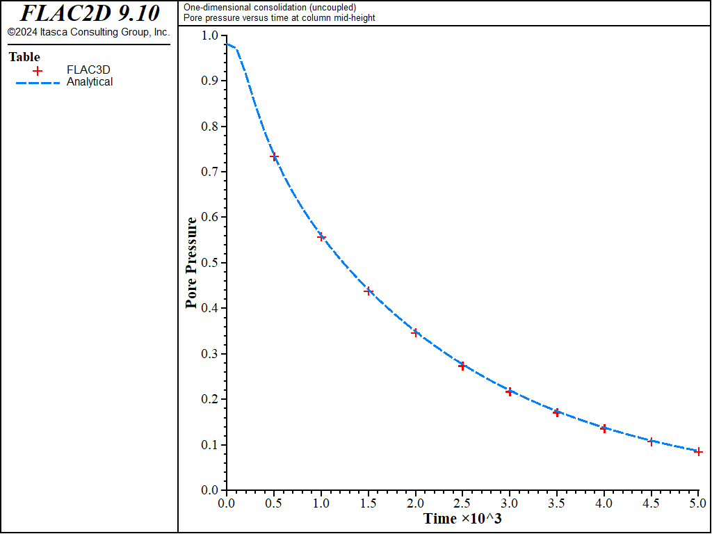
Figure 10: Comparison between analytical and numerical values of pore pressure in a 1D consolidation test - \(M\) = 4 × 10¹⁰ Pa.

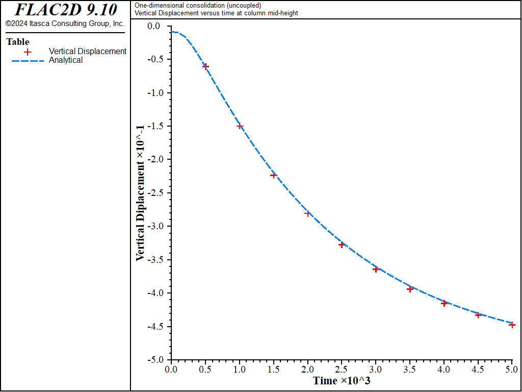
Figure 11: Comparison between analytical and numerical values for vertical displacement in a 1D consolidation test - \(M\) = 4 × 10¹⁰ Pa.

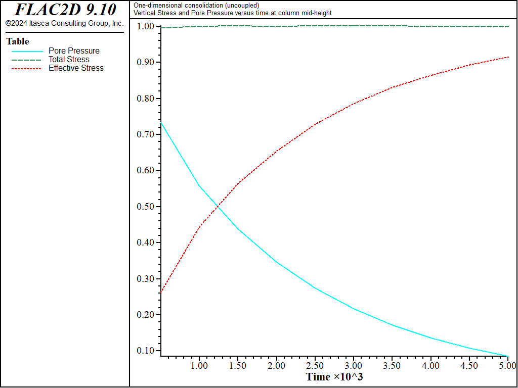
Figure 12: Evolution of pore pressure, total and effective stresses in a 1D consolidation test - \(M\) = 4 × 10¹⁰ Pa.

The uncoupled method switches calculations between fluid and matrix mechanical using the model solve-fluid-decoupled command. The results using the above simplified uncoupled method are presented in Figure Figure #fig1dconsolidation2d-simplified-pp to Figure Figure #fig1dconsolidation2d-simplified-evolution.

break

This particular example involves fully saturated coupled flow. In such cases, solution times can be reduced by using the saturated fast-flow algorithm described in Fully Saturated Fast Flow. The algorithm is selected by using the zone fluid fastflow on command. If 1DConsolidation-Coupled.dat with \(M\) = 4 × 10¹⁰ Pa (\(R_k\) = 52) is repeated with this command, the runtime is now approximately 12 seconds (see 1DConsolidation-FastFlow.dat). As \(R_k\) increases, the use of the fast-flow algorithm becomes more beneficial.

The results of the fast-flow calculation are shown in Figure 13 and Figure 14. The maximum relative error is less than 2%.

break

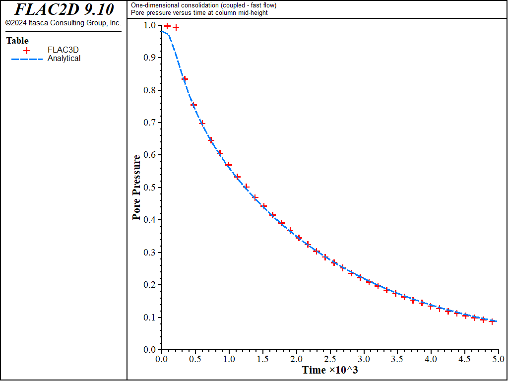
Figure 13: Comparison between analytical and numerical values of pore pressure in a 1D consolidation test.

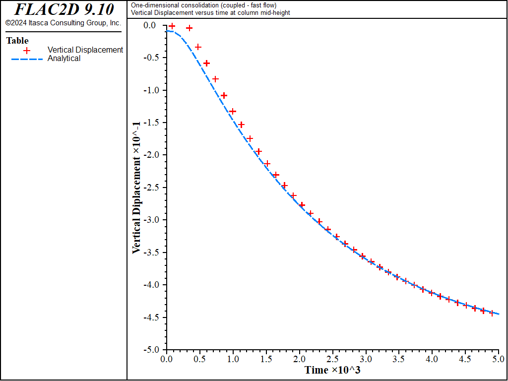
Figure 14: Comparison between analytical and numerical values for vertical displacement in a 1D consolidation test.

Reference

Detournay, E., and A. H. D. Cheng. “Fundamentals of Poroelasticity,” in Comprehensive Rock Engineering, Vol. 2, pp. 113-171. J. Hudson et al., eds. London: Pergamon Press (1993).

Data File

1DConsolidation-Coupled.dat

model new
model title "One-dimensional consolidation (coupled)"
; --- model geometry ---
zone create quadrilateral size 1 20
zone face skin
; --- mechanical model ---
model large-strain off
zone cmodel assign elastic
zone property bulk 5e8 shear 2e8
zone face apply velocity-normal 0 range group 'Top' not
zone face apply stress-normal -1e5 range group 'Top'
; --- fluid flow model ---
model configure fluid-flow
zone fluid property mobility-coefficient 1e-10 biot-modulus 4e9
zone fluid property pore-pressure-generation on
; --- first establish undrained response ---
model solve-static
; --- histories ---
history interval 10
zone history name="pp" pore-pressure position (0,10)
zone history name="syy" stress-yy position (0.5,10.5)
zone history name="ydisp" displacement-y position (0,10)
model history name="time" fluid time-total
; --- drained response ---
zone face apply pore-pressure 0 range group 'Top'
zone fluid implicit servo on 
model solve-fluid-coupled time 5000 convergence 1
model save '1dconsolidation_coupled'
program return

1DConsolidation-Coupled10M.dat

model new
model title "One-dimensional consolidation (coupled)"
; --- model geometry ---
zone create quadrilateral size 1 20
zone face skin
; --- mechanical model ---
model large-strain off
zone cmodel assign elastic
zone property bulk 5e8 shear 2e8
zone face apply velocity-normal 0 range group 'Top' not
zone face apply stress-normal -1e5 range group 'Top'
; --- fluid flow model ---
model configure fluid-flow
zone fluid property mobility-coefficient 1e-10 biot-modulus 4e10
zone fluid property pore-pressure-generation on
; --- first establish undrained response ---
model solve-static
; --- histories ---
history interval 10
zone history name="pp" pore-pressure position (0,10)
zone history name="syy" stress-yy position (0.5,10.5)
zone history name="ydisp" displacement-y position (0,10)
model history name="time" fluid time-total
; --- drained response ---
zone face apply pore-pressure 0 range group 'Top'
zone fluid implicit servo on 
model solve-fluid-coupled time 5000 convergence 1
model save '1dconsolidation_coupled_10M'
program return

1DConsolidation-Uncoupled.dat

model new
model title "One-dimensional consolidation (uncoupled)"
; --- model geometry ---
zone create quadrilateral size 1 20
zone face skin
; --- mechanical model ---
model large-strain off
zone cmodel assign elastic
zone property bulk [5e8+4e10] shear 2e8
zone face apply velocity-normal 0 range group 'Top' not
zone face apply stress-yy -1e5 range group 'Top'
model solve convergence 1
zone property bulk 5e8
; --- fluid flow model ---
model configure fluid-flow
zone fluid property mobility-coefficient 1e-10 fluid-modulus 4e10
zone fluid modulus-scale
; This is 1e5/(confinedModulus*storage)
zone gridpoint initialize pore-pressure 98119.4
zone face apply pore-pressure 0 range group 'Top'
zone results pore-pressure
; --- histories ---
model solve-fluid-decoupled time 5000 convergence 2 ...
   stages 10 stage-result '1dconsolidation_uncoupled_'
model save '1dconsolidation_uncoupled'
program return

1DConsolidation-FastFlow.dat

model new
model title "One-dimensional consolidation (coupled - fast flow)"
; --- model geometry ---
zone create quadrilateral size 1 20
zone face skin
; --- mechanical model ---
model large-strain off
zone cmodel assign elastic
zone property bulk 5e8 shear 2e8
zone face apply velocity-normal 0.0 range group 'Top' not
zone face apply stress-normal -1e5 range group 'Top'
; --- fluid flow model ---
model configure fluid-flow
zone fluid property mobility-coefficient 1e-10
; --- fast flow setting ---
zone fluid fastflow on ; implies implicit off, pore pressure generation on
; --- first establish undrained response ---
model solve-static
; --- histories ---
zone history name="pp" pore-pressure position (0,10)
zone history name="syy" stress-yy position (0.5,10.5)
zone history name="ydisp" displacement-y position (0,10)
model history name="time" fluid time-total
; --- drained response ---
zone face apply pore-pressure 0 range group 'Top'
model solve-fluid-coupled time 5000 convergence 0.1
model save '1dconsolidation_fastflow'
program return