Unconfined Flow Toward a Riverbank (FLAC2D)
Problem Statement
Note
The project file for this example is available to be viewed/run in FLAC2D. The main data files used are shown at the end of this example. The remaining data files can be found in the project.
The purpose of this problem is to determine the length of the seepage face \(l\),in an inclined riverbank, knowing the location of a point, \(P\) , on the phreatic surface. The slope of the riverbank is at angle \(α\). The location of point \(P\) is defined by distances \(L\) and \(H\). Figure 1 illustrates the geometry. For this problem:.
\(L\) |
= 100 m |
\(H\) |
= 50 m |
\(α\) |
= 45 ◦ |
The following material properties are assumed.
hydraulic conductivity (\(KH\)) |
10−6 (m/sec) |
porosity (\(n\)) |
0.3 |
water density (\(ρw\)) |
1000 kg/m3 |
soil dry density (\(ρ\)) |
1 kg/m3 |
gravity (g) |
10 m/sec 2 |
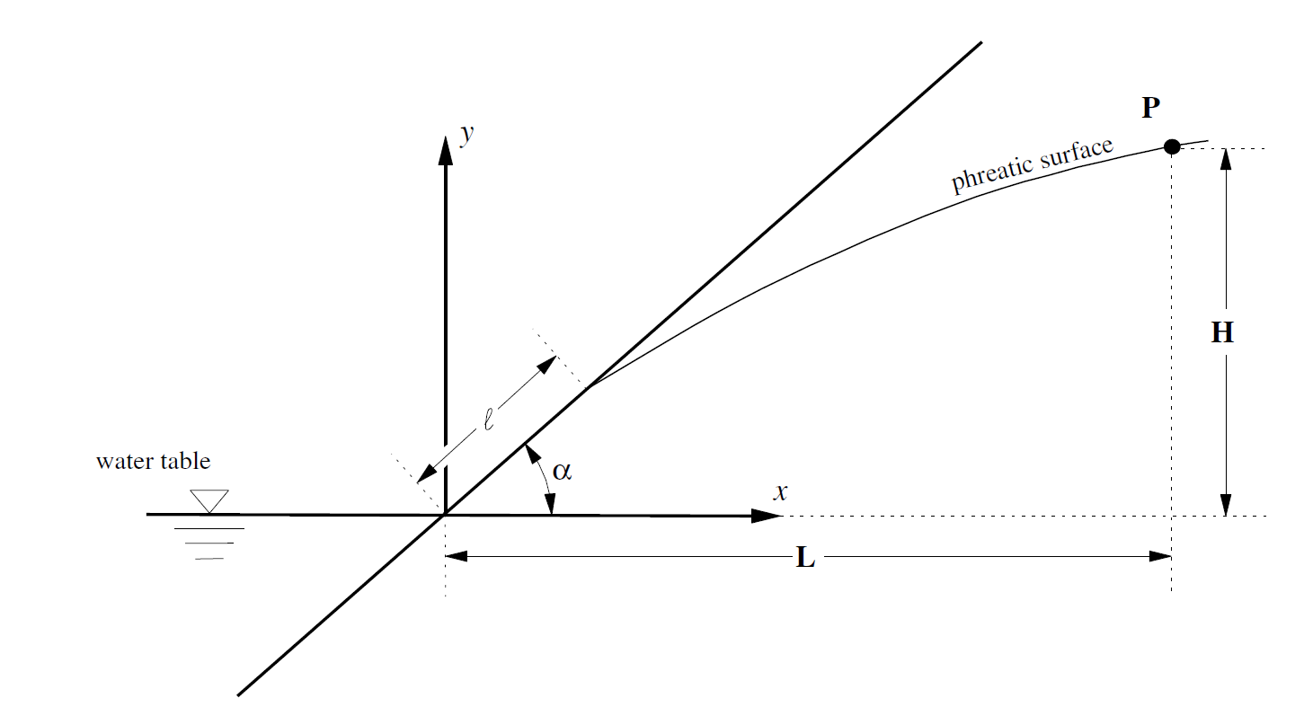
Figure 1: Problem geometry.
Closed-Form Solution
A closed-form solution to this problem based on the following assumptions is given by Strack and Asgian (1978).
The riverbank is represented as an infinite slope at an angle, α, with the horizontal.
Unconfined groundwater flows from far away toward the riverbank.
The flow is two-dimensional; no flow occurs in the direction parallel to the river.
The permeability is homogeneous and isotropic.
The flow is steady.
The soil is saturated below the phreatic surface and dry above it.
The solution is presented in the form of a chart given in Figure 2. This chart plots \(l/L\) as a function of \(H/L\) for different values of α. For this particular problem, \(H/L = 0.5\) and \(α = 45◦\), so \(l/L = 0.255\) and, since \(L = 100 m\), the length of the seepage face is \(l = 25.5 m\).
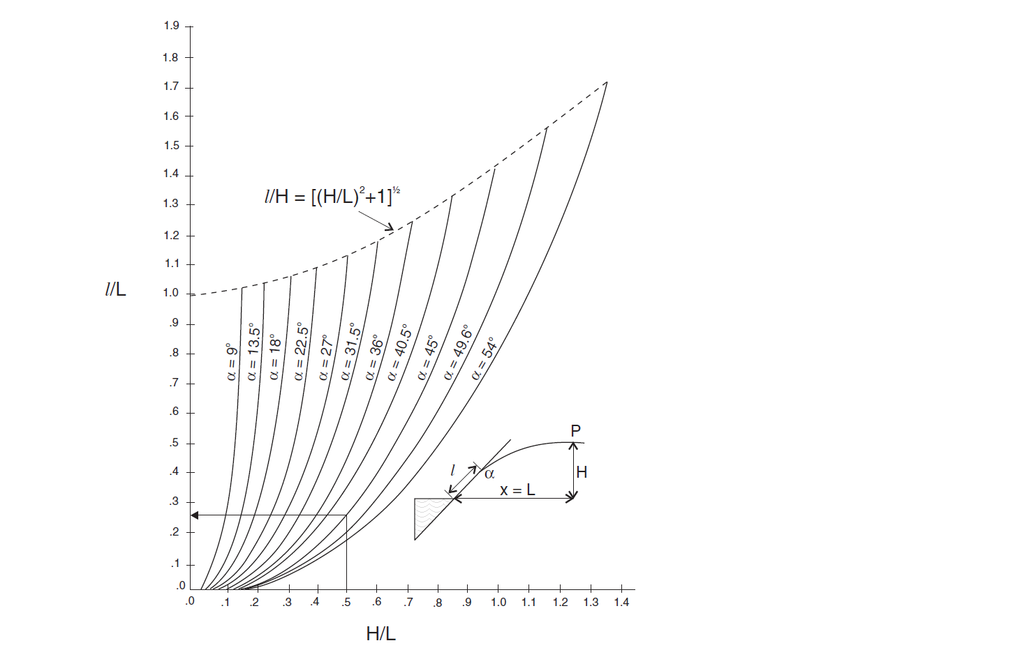
Figure 2: The seepage length, \(l\), as a function of the phreatic surface elevation, \(H\), at a point, \(P\), at a horizontal distance, \(L\), from the riverbank (adapted from Strack and Asgian 1978)
Figure 3 shows a flow net for α = 45 ◦.
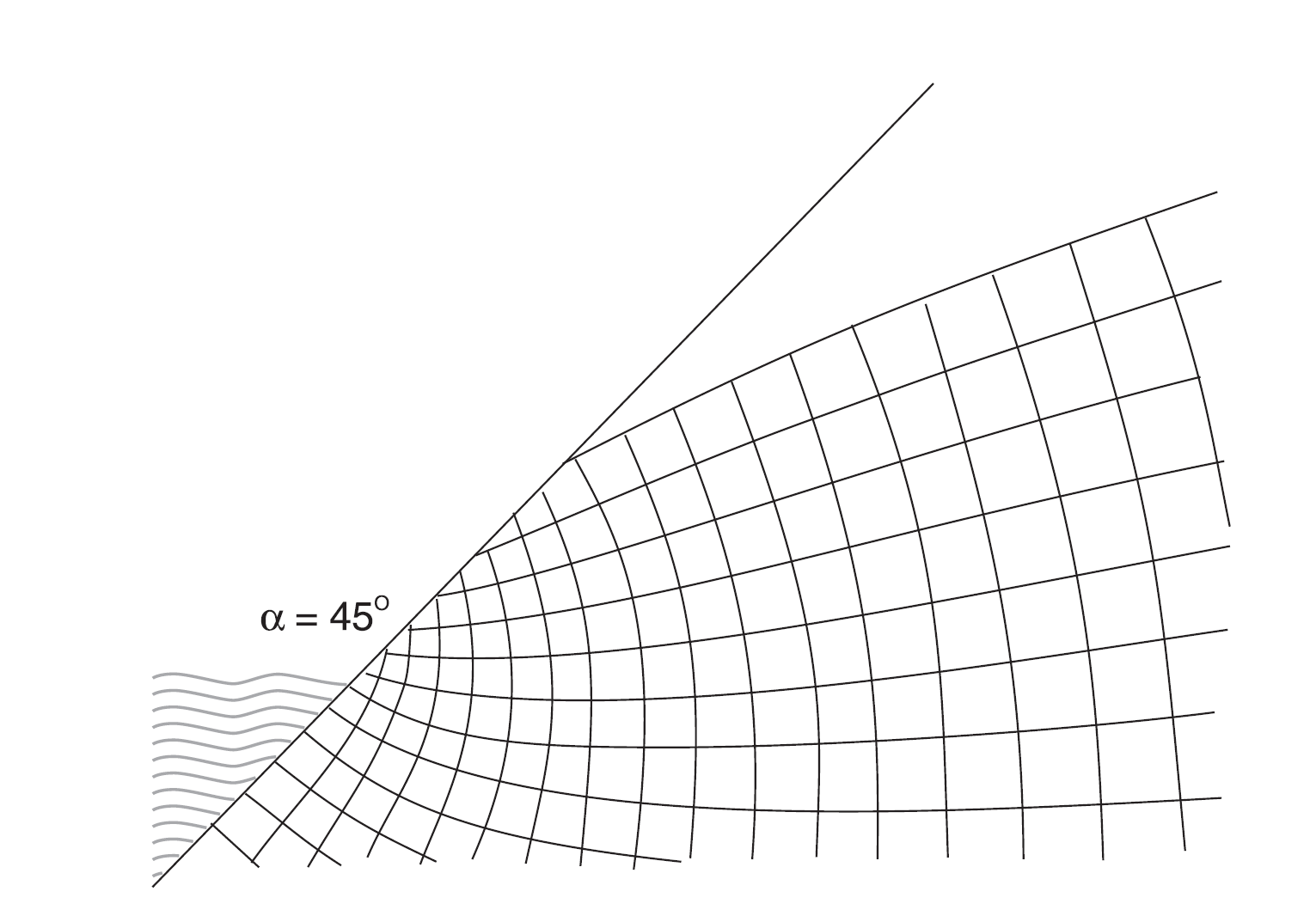
Figure 3: Flow net near the seepage face for α = 45 ◦ (Strack and Asgian 1978)
FLAC2D Model
A 30 × 40 grid is used, as shown in Figure 4. The fixed pore-pressure boundary conditions are also indicated on the figure. On the slope side of the model, the pore pressure follows a gravitational gradient for y <0 (below the river), and is zero for y >0. On the right side, the fixed pore pressure follows a gravitational gradient for −50 < y <50.
The material properties are assigned as described above. Because only the length of the seepage face under steady-state flow conditions is of interest, the actual values of the mechanical properties and homogeneous permeability are irrelevant.
Fist the model is solved with the zone fluid steady-state command. The model solves almost instantaneously.
The calculation is then repeated using the implicit flow solver. When a non steady-state solution is calculated, the fluid bulk modulus must be specified. Since the goal is to get to steady-state as quickly as possible, a fluid modulus less than the true modulus can be used. The modulus used is calculated from equation 12 of this document <Solving Flow-Only and Coupled-Flow Problems>.
The model solve-fluid command with a value of ratio-flow equal to 5e-3 is used to cycle the model to steady state. The evolution of the model is monitored using the FISH function “flow” , which calculates inflow and outflow at the fixed pore-pressure boundaries. At steady state, the free surface is a streamline,and inflow is equal to outflow.
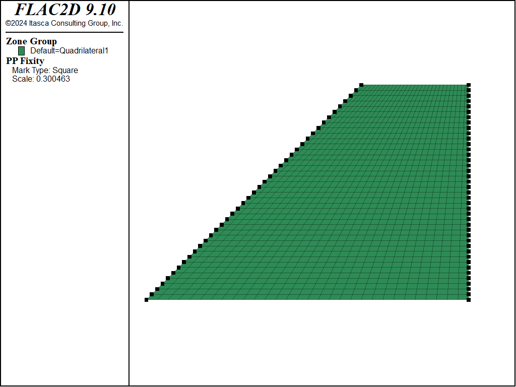
Figure 4: Zone geometry and fixed pore pressure gridpoints
Results and Discussion
The results are shown in Figures below (the steady state and implicit solution are virtually identical). The histories of inflow and outflow rates in Figure 5 indicate that a steady state of flow is indeed reached by the end of the implicit numerical simulation. Figure 6 shows the final flow vectors. Below the river’s surface,(y <0), the flow vectors are perpendicular to the slope face, which corresponds to an equipotential. Outflow occurs along the slope, and for some distance above the river level, but the flow vectors are not perpendicular to the slope’s surface. This is the calculated seepage face, and it compares closely with the analytical solution sketched on the figure.
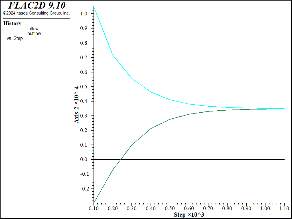
Figure 5: History of inflow and outflow
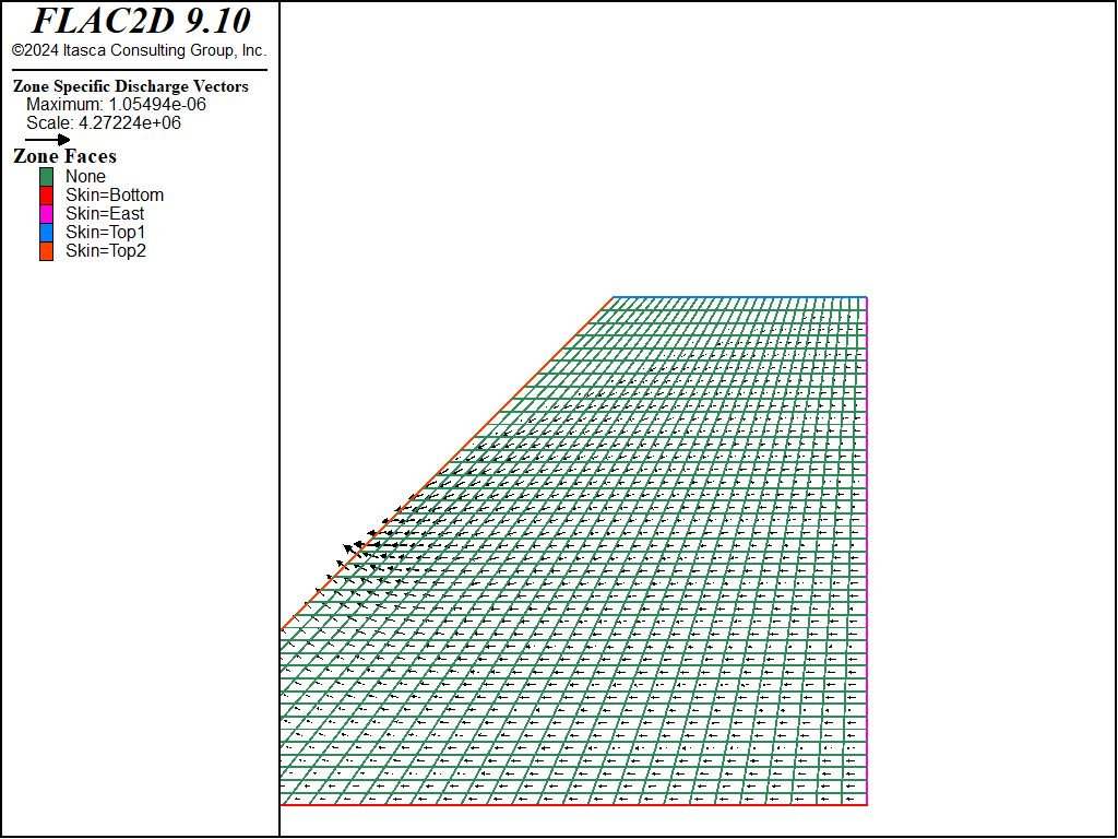
Figure 6: Steady-state flow vectors and seepage face solution
Reference
Strack, O. D. L., and M. I. Asgian. “A New Function for Use in the Hodograph Method,” \(Water Resources Research\), 14(6), 1045-1058 (1978).
Data Files
UnconfinedflowRiverbank.dat
;--------------------------------------------
;   Unconfined Flow toward a Riverbank
;--------------------------------------------
model new
model large-strain off
model configure fluid-flow
model gravity  0 -10

; Create zones
;zone import 'out' ; from FLAC 8.1

zone create2d quadrilateral point 0 -50,-50 point 1 100,-50 point 2 50,50 ...
  point 3 100,50 size 30 40

; Assign constitutive model and properties
zone cmodel assign elastic
zone property bulk 1.0 shear 1.0 density 1.0

; --- fluid properties ---
zone fluid property hydraulic-conductivity 1e-6 porosity 0.3
zone fluid-density 1000
zone fluid saturation cutoff

;boundary conditions
zone face skin
zone face apply head 50 datum 0,-50 range group 'Top2'  ; note group name!
zone face apply pore-pressure 0 range group 'Top2' position-y 0 50
zone face apply head 100 datum 0,-50 range group 'East'

; --- Settings ---
model gravity 10

model save 'initial'

; solve with steady state
zone fluid steady-state
model save 'steady-state'

========================================

; now solve with implicit solver
model restore 'initial'

zone fluid implicit on

zone fluid property fluid-modulus [0.3*1*1000*10/0.3] ; eqn 12

; --- Fish functions ---
[global pnt1= list(gp.list)(gp.isgroup(::gp.list,"East"))]
[global pnt2 =list(gp.list)(gp.isgroup(::gp.list,"Top2"))]
fish define flow
  global inflow
  global outflow
  global qratio
  inflow =list.sum(gp.flow(::pnt1))
  outflow =-1.0*list.sum(gp.flow(::pnt2))
 if (inflow + outflow) # 0.0 then
   qratio = 2.0 * math.abs(inflow - outflow) / (inflow + outflow)
 else
   qratio = 0.0
 end_if
end

; --- Histories ---
history interval 100
fish history flow
fish history name 'unbalanced ratio' qratio
fish history name 'inflow' inflow
fish history name 'outflow' outflow

; --- Solve ---
model solve-fluid ratio-flow  5e-3
model save 'rb1'
| Was this helpful? ... | Itasca Software © 2024, Itasca | Updated: Aug 13, 2024 |
