FLAC3D Modeling • Problem Solving with FLAC3D
Material Properties
The material properties required in FLAC3D are generally categorized in one of two groups: elastic deformability properties and strength properties. This section provides an overview of the deformability and strength properties, and presents guidelines for selecting the appropriate properties for a given model. Additionally, there are special considerations, such as the definition of post-failure properties, the extrapolation of laboratory-measured properties to the field scale, the spatial variation of properties and randomness of the property distribution, and the dependence of properties on confinement and strain. These topics are also discussed.
The selection of properties is often the most difficult element in the generation of a model because of the high uncertainty in the property database. When performing an analysis, especially in geomechanics, keep in mind that the problem will always involve a data-limited system: the field data will never be known completely. However, with the appropriate selection of properties based upon the available database, important insight to the physical problem can still be gained. This approach to modeling was discussed earlier in Modeling Methodology.
Material properties are conventionally derived from laboratory testing programs. The following sections describe intrinsic (laboratory-scale) properties and list common values for various rocks and soils.
Intrinsic Deformability Properties
Isotropic Elastic Properties — All material models in FLAC3D, except for the transversely isotropic elastic and orthotropic elastic models, assume an isotropic material behavior in the elastic range described by two elastic constants: bulk modulus (\(K\)) and shear modulus (\(G\)). The elastic constants, \(K\) and \(G\), are preferred rather than Young’s modulus, \(E\), and Poisson’s ratio, \(ν\). While both can be used in FLAC3D, it is believed that bulk and shear moduli correspond to more fundamental aspects of material behavior than do Young’s modulus and Poisson’s ratio. (See tip 13. Use Bulk and Shear Moduli in the topic Tips and Advice for justification of using (\(K,G\)) rather than (\(E,ν\)).)
The equations to convert from (\(E,ν\)) to (\(K,G\)) are
The equations above should be used with caution when \(ν\) is near 0.5, because the computed value of \(K\) will be unrealistically high and convergence to the solution will be very slow. It is better to fix the value of \(K\) at its known physical value (estimated from an isotropic compaction test or from the \(p\)-wave speed), and then compute \(G\) from \(K\) and \(ν\).
Some typical values for elastic constants are summarized in the next table for selected rocks and in the table following for selected soils.
Dry Density (kg/m 3 ) |
\(E\) (GPa) |
\(ν\) |
\(K\) (GPa) |
\(G\) (GPa) |
|
|---|---|---|---|---|---|
sandstone |
19.3 |
0.38 |
26.8 |
7.0 |
|
siltstone |
26.3 |
0.22 |
15.6 |
10.8 |
|
limestone |
2090 |
28.5 |
0.29 |
22.6 |
11.1 |
shale |
2210 - 2570 |
11.1 |
0.29 |
8.8 |
4.3 |
marble |
2700 |
55.8 |
0.25 |
37.2 |
22.3 |
granite |
73.8 |
0.22 |
43.9 |
30.2 |
Dry Density (kg/m 3) |
Elastic Modulus \(E\) (MPa) |
Poisson’s Ratio |
|
|---|---|---|---|
loose uniform sand |
1470 |
10 - 26 |
0.2 - 0.4 |
dense uniform sand |
1840 |
34 - 69 |
0.3 - 0.45 |
loose, angular-grained, silty sand |
1630 |
||
dense, angular-grained, silty sand |
1940 |
0.2 - 0.4 |
|
stiff clay |
1730 |
6 - 14 |
0.2 - 0.5 |
soft clay |
1170 - 1490 |
2 - 3 |
0.15 - 0.25 |
loess |
1380 |
||
soft organic clay |
610 - 820 |
||
glacial till |
2150 |
Anisotropic Elastic Properties — For the special case of elastic anisotropy, the transversely isotropic, elastic model requires five elastic constants: \(E_1\), \(E_3\), \(\nu_{12}\), \(\nu_{13}\), and \(G_{13}\); and the orthotropic elastic model requires nine elastic constants: \(E_1\), \(E_2\), \(E_3\), \(\nu_{12}\), \(\nu_{13}\), \(\nu_{23}\), \(G_{12}\), \(G_{13}\), and \(G_{23}\). These constants are defined in Orthotropic Elastic Model**.
Transversely isotropic elastic behavior is commonly associated with uniformly jointed or bedded rock. Several investigators have developed expressions for the elastic constants in terms of intrinsic isotropic elastic properties and joint stiffness and spacing parameters. A short summary of typical values for anisotropic rocks is given in the following table.
Rock |
\(E_x\) (GPa) |
\(E_y\) (GPa) |
\(ν_{yx}\) |
\(ν_{zx}\) |
\(G_{xy}\) (GPa) |
|---|---|---|---|---|---|
siltstone |
43.0 |
40.0 |
0.28 |
0.17 |
17.0 |
sandstone |
15.7 |
9.6 |
0.28 |
0.21 |
5.2 |
limestone |
39.8 |
36.0 |
0.18 |
0.25 |
14.5 |
gray granite |
66.8 |
49.5 |
0.17 |
0.21 |
25.3 |
marble |
68.6 |
50.2 |
0.06 |
0.22 |
26.6 |
sandy shale |
10.7 |
5.2 |
0.20 |
0.41 |
1.2 |
Fluid Elastic Properties — Models created for groundwater analysis also require the bulk modulus of the water, \(K_f\), if the calculation involves incompressible grains, or the Biot modulus, \(M\), if the grains are compressible. The physical value of \(K_f\) is 2 GPa for pure water at room temperature. The value selected should depend on the purpose of the analysis. If only steady-state flow or an initial pore pressure distribution is required (see Solving Flow-Only and Coupled-Flow Problems), then as low a value of \(K_f\) as possible should be used, without compromising the physics. This is because the fluid timestep will be small for high \(K_f\); also, the mechanical convergence will be very slow for high \(K_f\). The fluid timestep, \(Δt_f\), used by FLAC3D is related to porosity, \(n\), permeability, \(k'\), and \(K_f\):
We can determine the effect of changing \(K_f\) by deriving the coefficient of consolidation, \(C_v\), for the case of a deformable fluid. (The fluid is assumed incompressible in most textbook solutions.)
where
and
where: |
\(k'\) |
= |
permeability used in FLAC3D; |
\(k\) |
= |
hydraulic conductivity in velocity units (e.g., m/sec); and |
|
\(\gamma_f\) |
= |
the unit weight of water. |
Because the consolidation time constant is directly proportional to \(C_v\), the expression allows us to see how much error is introduced by reducing \(K_f\) from its real value (of 2 × 10⁹ Pa).
The fluid bulk modulus will also affect the rate of convergence for a model with no flow, but with mechanical generation of pore pressure (see No Flow — Mechanical Generation of Pore Pressure). If \(K_f\) is given a value comparable to the mechanical moduli, pore pressures will be generated as a result of mechanical deformations. If \(K_f\) is much greater than \(K\), then convergence will be slow, but often it is possible to reduce \(K_f\) without significantly affecting the behavior. In real soils, for example, pore water will contain some dissolved air, which substantially reduces its apparent bulk modulus.
In the case of no flow, the undrained saturated bulk modulus is
and the undrained Poisson’s ratio is
These values should be compared to the drained constants \(K\) and \(ν\) to evaluate the effect on the rate of convergence. It is important to remember that drained properties are used for coupled, mechanical fluid-flow calculations in FLAC3D.
For the case of compressible grains, the influence of Biot modulus, \(M\), on the rate of convergence for a model is similar to that of fluid bulk modulus.
Intrinsic Strength Properties
The basic criterion for material failure in FLAC3D is the Mohr-Coulomb relation, which is a linear failure surface corresponding to shear failure:
where: |
\(N_\phi\) |
= |
\((1+\sin \phi) / (1-\sin \phi)\); |
\(\sigma_1\) |
= |
major principal stress (compressive stress is negative); |
|
\(\sigma_3\) |
= |
minor principal stress; |
|
\(\phi\) |
= |
friction angle; and |
|
\(c\) |
= |
cohesion. |
Shear yield is detected if \(f_s\) < 0. The two strength constants, \(\phi\) and \(c\), are conventionally derived from laboratory triaxial tests.
The Mohr-Coulomb criterion loses its physical validity when the normal stress becomes tensile, but for simplicity, the surface is extended into the tensile region to the point at which \(\sigma_3\) equals the uniaxial tensile strength, \(\sigma^t\). The minor principal stress can never exceed the tensile strength, i.e.,
Tensile yield is detected if \(f_t\) > 0. Tensile strengths from rock and concrete are usually derived for a Brazilian test. Note that the tensile strength cannot exceed the value of \(\sigma_3\), corresponding to the apex limit for the Mohr-Coulomb relation. This maximum value is given by
Typical values of cohesion, friction angle and tensile strength for a representative set of rock specimens are listed in the next table. Cohesion and friction angle values for soil specimens are given in the table following. Strength is often described in terms of the unconfined compressive strength, \(q_u\). The relation between \(q_u\) and cohesion, \(c\), and friction angle, \(\phi\), is given by
Friction Angle (degrees) |
Cohesion (MPa) |
Tensile Strength (MPa) |
|
|---|---|---|---|
Berea sandstone |
27.8 |
27.2 |
1.17 |
Repetto siltstone |
32.1 |
34.7 |
— |
Muddy shale |
14.4 |
38.4 |
— |
Sioux quartzite |
48.0 |
70.6 |
— |
Indiana limestone |
42.0 |
6.72 |
1.58 |
Stone Mountain granite |
51.0 |
55.1 |
— |
Nevada Test Site basalt |
31.0 |
66.2 |
13.1 |
Cohesion (kPa) |
Friction Angle Peak (degrees) |
Residual (degrees) |
|
|---|---|---|---|
gravel |
— |
4 |
32 |
sandy gravel with few fines |
— |
35 |
32 |
sandy gravel with silty or clayey fines |
1.0 |
35 |
32 |
mixture of gravel and sand with fines |
3.0 |
28 |
22 |
uniform sand — fine |
— |
32 |
30 |
uniform sand — coarse |
— |
34 |
30 |
well-graded sand |
— |
33 |
32 |
low-plasticity silt |
2.0 |
28 |
25 |
medium- to high-plasticity silt |
3.0 |
25 |
22 |
low-plasticity clay |
6.0 |
24 |
20 |
medium-plasticity clay |
8.0 |
20 |
10 |
high-plasticity clay |
10.0 |
17 |
6 |
organic silt or clay |
7.0 |
20 |
15 |
Drucker-Prager strength parameters can be estimated from cohesion and friction angle properties. For example, assuming that the Drucker-Prager failure envelope circumscribes the Mohr-Coulomb envelope, the Drucker-Prager parameters \(q_{\phi}\) and \(k_{\phi}\) are related to \(\phi\) and \(c\) by
For further explanation on the relations between Drucker-Prager model parameters, see Notes on Parameters.
The ubiquitous-joint model also requires strength properties for the planes of weakness. Joint properties are conventionally derived from laboratory testing (e.g., triaxial and direct shear tests). These tests can produce physical properties for joint friction angle, cohesion, dilation angle, and tensile strength.
Published strength properties for joints can be found, for example, in Jaeger and Cook (1969), Kulhawy (1975), and Barton (1976). Friction angles can vary from less than 10° for smooth joints in weak rock, such as tuff, to over 50° for rough joints in hard rock, such as granite. Joint cohesion can range from zero cohesion to values approaching the compressive strength of the surrounding rock.
It is important to recognize that joint properties measured in the laboratory typically are not representative of those for real joints in the field. Scale-dependence of joint properties is a major question in rock mechanics. Often, comparison to similar joint properties derived from field tests is the only way to guide the choice of appropriate parameters. However, field test observations are extremely limited. Some results are reported by Kulhawy (1975).
Post-Failure Properties
In many instances, particularly in mining engineering, the response of a material after failure has initiated is an important factor in the engineering design. Consequently, the post-failure behavior must be simulated in the material model. In FLAC3D, this is accomplished with properties that define four types of post failure response:
shear dilatancy;
shear hardening/softening;
volumetric hardening/softening; and
tensile softening.
These properties are only activated after failure is initiated, as defined by the Mohr-Coulomb relation or the tensile-failure criterion. Shear dilatancy is simulated with the Mohr-Coulomb, ubiquitous-joint and strain-softening Mohr-Coulomb and ubiquitous-joint models. Shear hardening/softening is simulated with the strain-softening Mohr-Coulomb and ubiquitous-joint models, and volumetric hardening/softening is simulated with the modified Cam-clay model. Tensile softening is simulated with the strain-softening Mohr-Coulomb and ubiquitous-joint models.
Shear Dilatancy
Shear dilatancy, or dilatancy, is the change in volume that occurs with shear distortion of a material. Dilatancy is characterized by a dilation angle, \(\psi\), which is related to the ratio of plastic volume change to plastic shear strain. This angle can be specified in the Mohr-Coulomb ubiquitous-joint and strain-hardening/softening models in FLAC3D. Dilation angle is typically determined from triaxial tests or shear-box tests. For example, the idealized relation for dilatancy, based upon the Mohr-Coulomb failure surface, is depicted for a triaxial test in the figure below. The dilation angle is found from the plot of volumetric strain versus axial strain. Note that the initial slope for this plot corresponds to the elastic regime, while the slope used to measure the dilation angle corresponds to the plastic regime.
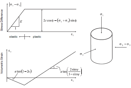
Figure 1: Idealized relation for dilation angle, \(\psi\), from triaxial test results (Vermeer and de Borst 1984).
For soils, rocks, and concrete, the dilation angle is generally significantly smaller than the friction angle of the material. Vermeer and de Borst (1984) report the following typical values for \(\psi\).
dense sand |
15° |
loose sand |
< 10° |
normally consolidated clay |
0° |
granulated and intact marble |
12°–20° |
concrete |
12° |
Vermeer and de Borst observe that values for the dilation angle are approximately between 0° and 20°, whether the material is soil, rock, or concrete. The default value for dilation angle is zero for all the constitutive models in FLAC3D.
Dilation angle can also be prescribed for the joints in the ubiquitous-joint model. This property is typically determined from direct shear tests, and common values can be found in the references discussed in Intrinsic Strength Properties.
Shear Hardening/Softening
The initiation of material hardening or softening is a gradual process once plastic yield begins. At failure, deformation becomes more and more inelastic as a result of micro-cracking in concrete and rock, and particle sliding in soil. This also leads to degradation of strength in these materials and the initiation of shear bands. These phenomena, related to localization, are discussed in Modeling Methodology.
In FLAC3D, shear hardening and softening are simulated by making Mohr-Coulomb properties (cohesion and friction, along with dilation) functions of plastic strain (see Strain-Softening/Hardening Mohr-Coulomb (SSoft) Model). These functions are accessed from the strain-softening model, and can be specified either with a table or via a FISH function.
Hardening and softening parameters must be calibrated for each specific analysis, and the values are generally back-calculated from results of laboratory triaxial tests. This is usually an iterative process. Investigators have developed expressions for hardening and softening. For example, Vermeer and de Borst (1984) propose the frictional hardening relation
where |
\(\phi\) |
= |
ultimate friction angle; |
\(\phi_m\) |
= |
mobilized friction angle; |
|
\(e_p\) |
= |
plastic strain; and |
|
\(e_f\) |
= |
parameter. |
Cundall (1989) incorporates this relation into two-dimensional FLAC to study localization in a frictional material. This is accomplished by approximating the function with a table relating friction angle to plastic strain (i.e., table accessed from zone property table-friction). This approach is demonstrated for the Compression test on strain-softening material example described previously.
Numerical testing conditions can influence the model response for shear hardening/softening behavior. The rate of loading can introduce inertial effects. The results are also grid-dependent. Thus, it is important to evaluate the model behavior for differing zone size and grid orientation whenever performing an analysis involving shear hardening or softening.
The following example illustrates the application of a shear-softening material in a uniaxial compression test. A low velocity is applied to the top and bottom of the specimen, and the grid contains fine zoning. The softening response is shown in the stress-displacement plot in the next figure. The development of localization and shear bands can be observed in the second and third figure following. The plastic region is identified as hourglass-shaped with spiral structures radiating from the hourglass cones.
Uniaxial test of a shear-softening material
; Uniaxial test of strain-softening material
model new
model large-strain off
model title 'Uniaxial test of strain-softening material'
; Create zones
zone create cylinder point 0 (0,0,0) point 1 (1,0,0) ...
                     point 2 (0,4,0) point 3 (0,0,1) ...
                     size 12 30 12
zone reflect normal (1,0,0)
zone reflect normal (0,0,1)
zone face skin
; Constitutive model and properties
zone cmodel assign strain-softening
zone property density 2500 bulk 2e8 shear 1e8
zone property cohesion 2e6 friction 45 tension 2e5 dilation 10
zone property table-friction 'fri' table-cohesion 'coh' table-dilation 'dil'
table 'fri' add (0, 45) (.05, 42) (.1, 40) (1, 40)
table 'coh' add (0,2e6) (.05,1e6) (.1,5e5) (1,5e5)
table 'dil' add (0, 10) (.05,  3) (.1,  0)
; Boundary Conditions
zone face apply velocity (0,-2.5e-5,0) range group 'North'
zone face apply velocity (0, 2.5e-5,0) range group 'South'
; Histories
history interval 1
zone history displacement-y position (0,0,0)
zone history displacement-x position (1,1,0)
; FISH to store gridpoints on y=0 surface 'South'
fish define FindSurface
    global surface = map
    loop foreach local gp gp.list
        if gp.isgroup(gp,'South') then
            surface(gp.id(gp)) = gp
        endif
    endloop
end
[FindSurface]
; FISH to track AxialStress on y=0 surface 'South'
fish define AxialStress
    local str = 0
    loop foreach local gp surface
        str = str + gp.force.unbal.y(gp)
    endloop
    AxialStress = str / math.pi   ;  cylinder radius = 1
end
fish history AxialStress
model step 5000
; Plot of plastic region as zones with strain > 0.2
fish define TagPlasticZones
    loop foreach local zp zone.list
        if zone.prop(zp,'strain-shear-plastic') > 0.2
            zone.group(zp) = 'Yield'
        else
            zone.group(zp) = 'Other'
        endif
    endloop
end
[TagPlasticZones]
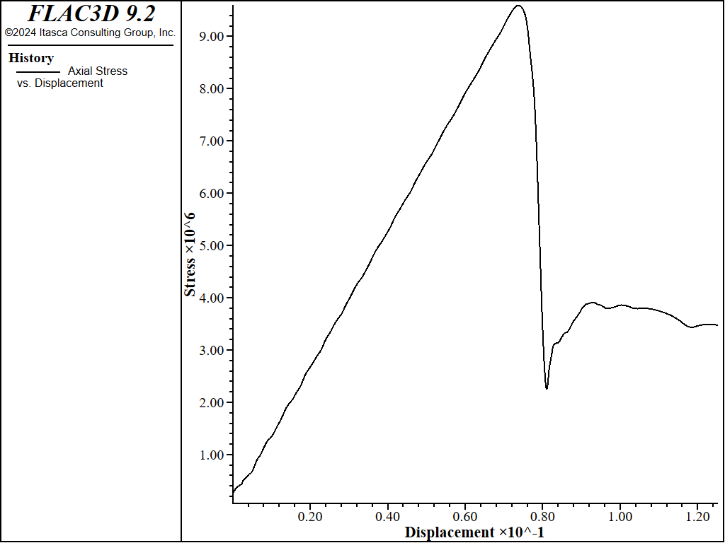
Figure 2: Stress-displacement plot for uniaxial test of shear-softening material
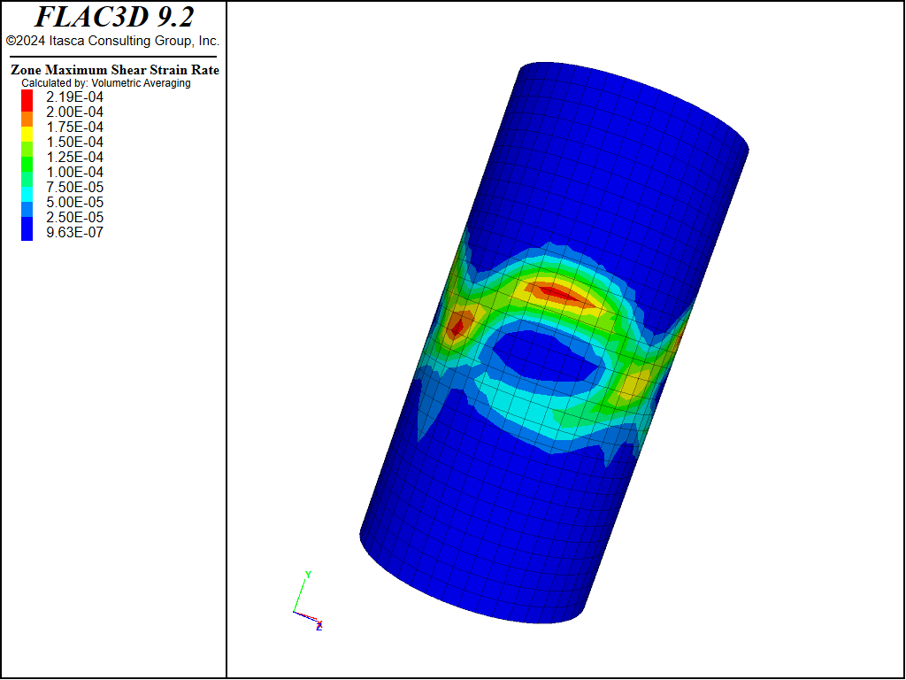
Figure 3: Contours of shear-strain rate indicating shear bands in strain-softening material.
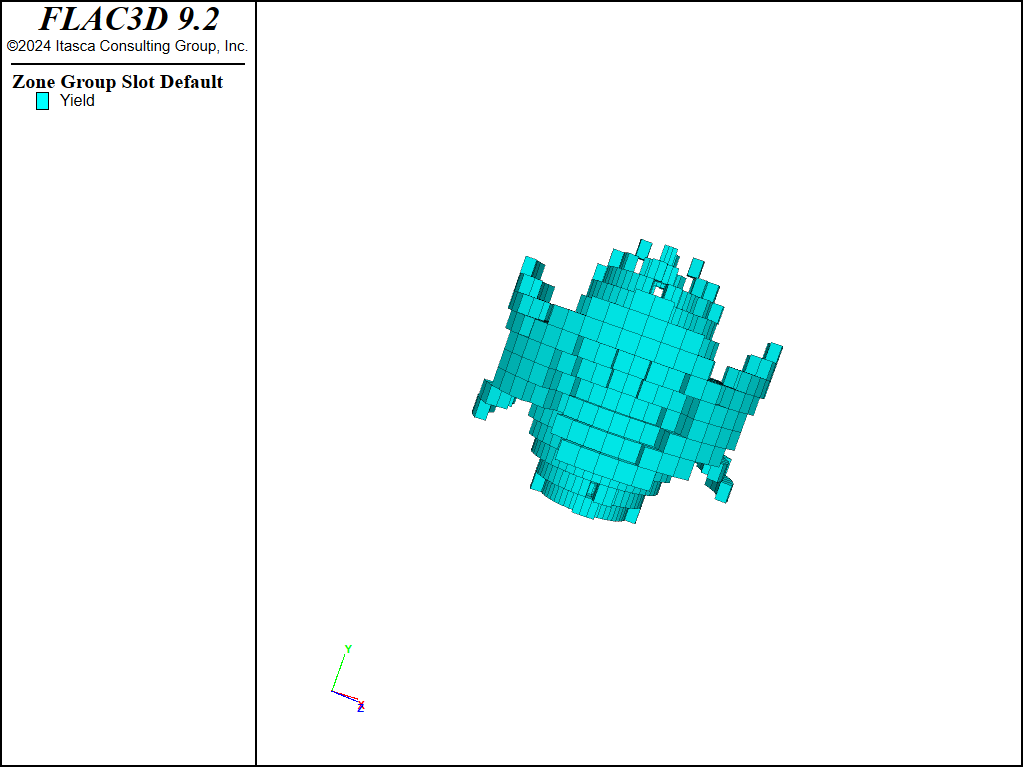
Figure 4: Yielded region identified as zones with plastic shear strain > 0.2.
Volumetric Hardening/Softening
Volumetric hardening corresponds to irreversible compaction; increasing the isotropic pressure can cause permanent volume decrease. This behavior is common in materials such as lightly cemented sands and gravels and over-consolidated clays.
Volumetric hardening/softening may be simulated in the double-yield model and the Cam-clay model. The double-yield model assumes that the hardening depends on plastic volume strain, while the Cam-clay model treats volumetric hardening as a function of both shear and volume strain.
The double-yield model takes its hardening rule from either a table or a FISH function. This example describes a recommended test procedure to develop these parameters from triaxial tests performed at constant mean stress, and for loading in which axial stress and confining pressure are kept equal. Typically, though, these data are not available. An alternative is to back-calculate the parameters from a uniaxial strain (or oedometer) test.
The modified Cam-clay model is defined by initial elastic moduli plus parameters that prescribe the nonlinear elasticity and hardening/softening behavior. The properties include the following:
\(\kappa\) |
slope of the elastic swelling line |
\(\lambda\) |
slope of the normal consolidation line |
\(M\) |
material constant |
\(p_c\) |
pre-consolidation pressure |
\(p_1\) |
reference pressure |
\(v_0\) |
initial specific volume |
\(v_{\lambda}\) |
specific volume at reference pressure on normal consolidation line |
The definition of these properties can be found in soil mechanics texts (e.g., Wood 1990). The procedures for determining these properties from laboratory tests are described in Determination of Input Parameters. It is recommended that single-zone tests be conducted with FLAC3D to exercise the modified Cam-clay model, and verify whether the choice of model properties is adequate. An example test is provided in the isotropic consolidation example.
Tensile Softening
At the initiation of tensile failure, the tensile strength of a material will generally drop to zero. The rate at which the tensile strength drops, or tensile softening occurs, is controlled by the plastic tensile strain in FLAC3D. This function is accessed from the strain-softening model and can be specified either with a table or via a FISH function.
A simple tension test illustrates the tensile-softening behavior. The model is the same as that used previously in the compression test on Mohr-Coulomb material and the compression test on strain-softening material in the topic Selection of an Appropriate Model. The ends of the cylindrical sample are now pulled apart at a constant velocity.
Tension test on tensile-softening material
model new
model large-strain off
; Create zones
zone create cylinder point 0 (0,0,0) point 1 (1,0,0) ...
                     point 2 (0,2,0) point 3 (0,0,1) ...
                     size 4 5 4
zone reflect normal (1,0,0)
zone reflect normal (0,0,1)
zone face skin
; Assign constitutive model and properties
zone cmodel assign strain-softening
zone property bulk 1.19e10 shear 1.1e10
zone property cohesion 2.72e5 friction 44 tension 2e5
zone property table-tension 'ten'
table 'ten' add (0,2e5) (2e-5,0)
; Boundary conditions
zone face apply velocity (0, 1e-8,0) range group 'North'
zone face apply velocity (0,-1e-8,0) range group 'South'
; Histories
history interval 1
zone history displacement-y position (0,0,0)
zone history displacement-x position (1,1,0)
; FISH to store gridpoints on y=0 surface 'South'
fish define FindSurface
    global surface = map
    loop foreach local gp gp.list
        if gp.isgroup(gp,'South') then
            surface(gp.id(gp)) = gp
        endif
    endloop
end
[FindSurface]
; FISH to track AxialStress on y=0 surface 'South'
fish define AxialStress
    local str = 0
    loop foreach local gp surface
        str = str + gp.force.unbal.y(gp)
    endloop
    AxialStress = str / math.pi   ;  cylinder radius = 1
end
fish history AxialStress
model step 1500
The plot of axial stress versus axial displacement (the next figure) shows that the average axial stress through the center of the model drops to zero. (The stress will remain constant in the non-softening Mohr-Coulomb model.) The model decreases in diameter until tensile failure initiates, then expands as tensile softening occurs (see the second figure below). The brittleness of the tensile softening is controlled by the plastic tensile-strain function. As with the shear hardening/softening model, the tensile-softening model must be calibrated for each specific problem and grid size.
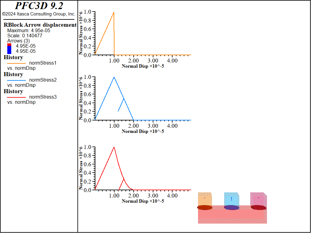
Figure 5: Axial stress versus axial displacement for tensile test of tension-softening material.
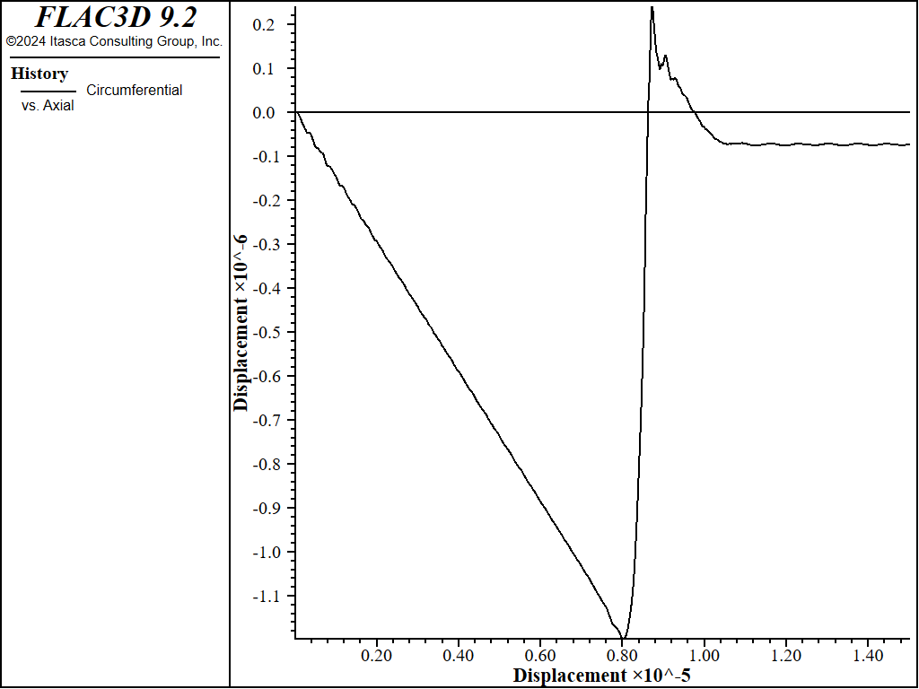
Figure 6: Circumferential displacement versus axial displacement for tensile test of tension-softening material.
Volume-Pressure Properties
The double-yield and modified Cam-clay models require material properties that relate pressure to volumetric change. For both models, the pre-consolidation pressure is the maximum past consolidation pressure. In the double-yield model, the relation between pressure and volumetric change is expressed by a table relating the cap pressure to plastic volume strain. In the Cam-clay model, the pressure-volume relation is expressed by the slopes of the initial compression line and the reloading-unloading line for the plot of volumetric strain versus natural log of pressure. The recommended procedure for selecting volumetric properties for the double-yield model is given in Choice of Volumetric Properties; the procedure for the Cam-clay model is given in Implementation Procedure.
Extrapolation to Field-Scale Properties
The material properties used in the FLAC3D model should correspond as closely as possible to the actual values of the physical problem. Particularly in rock, the laboratory-measured properties generally should not be used directly in a FLAC3D model for a full-scale problem. These properties should be scaled to account for the presence of discontinuities and heterogeneities present in a rock mass.
Several empirical approaches have been proposed to derive field-scale properties. Some of the more commonly accepted methods are discussed.
Deformability of a rock mass is generally defined by a modulus of deformation, \(E_m\). If the rock mass contains a set of relatively parallel, continuous joints with uniform spacing, the value for \(E_m\) can be estimated by treating the rock mass as an equivalent transversely isotropic continuum. The following relation can then be used to estimate \(E_m\) in the direction normal to the joint set.
where: |
\(E_m\) |
= |
rock mass Young’s modulus; |
\(E_r\) |
= |
intact rock Young’s modulus; |
|
\(k_n\) |
= |
joint normal stiffness; and |
|
\(s\) |
= |
joint spacing. |
A similar expression can be derived for shear modulus:
where: |
\(G\) |
= |
rock mass shear modulus; |
\(G_r\) |
= |
intact rock shear modulus; and |
|
\(k_s\) |
= |
joint shear stiffness. |
The equivalent continuum assumption, when extended to three orthogonal joint sets, produces the following relations:
Several expressions have been derived for two- and three-dimensional characterizations and multiple joint sets. References for these derivations can be found in Singh (1973), Gerrard (1982a and b), and Fossum (1985).
In practice, the rock mass structure is often much too irregular, or sufficient data are not available, to use the preceding approach. It is common to determine \(E_m\) from a force-displacement curve obtained from an in-situ compression test. Such tests include plate-bearing tests, flatjack tests, and dilatometer tests.
Bieniawski (1978) developed an empirical relation for \(E_m\) based upon field test results at sites throughout the world. The relation is based upon rock mass rating (RMR). For rocks with a rating higher than 55, the test data can be approximately fit to
The units of \(E_m\) are GPa.
For values of \(E_m\) between 1 and 10 GPa, Serafim and Pereira (1983) found a better fit, given by
References by Goodman (1980) and Brady and Brown (1985) provide additional discussion on these methods.
The most commonly accepted approach to estimate rock mass strength is that proposed by Hoek and Brown (1980). The generalized Hoek-Brown failure criterion for jointed rock masses is defined by (Hoek and Brown 1997):
where \(\sigma'_{1}\) and \(\sigma'_{3}\) are the maximum and minimum effective stress at failure, respectively (compressive stresses are positive), \(m_b\) is the value of the Hoek-Brown constant \(m\) for the rock mass, \(s\) and \(a\) are constants that depend upon the characteristics of the rock mass, and \(\sigma_{ci}\) is the uniaxial compressive strength of the intact rock pieces.
The tensile strength of the rock mass is estimated by Hoek and Brown (1997) to be
Three properties are required in order to use the Hoek-Brown criteria (Equations (1) and (2) above):
the uniaxial compressive strength, \(\sigma_{ci}\), of the intact rock pieces;
the Hoek-Brown constant, \(m_i\), for the intact rock pieces; and
the value of the Geological Strength Index, GSI, for the rock mass. This provides an estimate for the Hoek-Brown constants, \(s\), \(m_b\), and \(a\).
For the intact rock pieces that compose the rock mass, Equation (1) becomes
The values for \(\sigma_{ci}\) and the constant \(m_i\) should be determined by statistical analysis of the results of a set of triaxial tests. The recommended procedure is given by Hoek and Brown (1997). This paper also presents estimates of \(\sigma_{ci}\) and \(m\) for preliminary design calculations when laboratory test results may not be available.
The Geological Strength Index (GSI) provides a system for estimating the reduction in rock mass strength. Two tables from Hoek and Brown (1997) can be used to estimate GSI (see the two tables below). Hoek and Brown (1997) then give the following relation between GSI and \(m_b\), \(s\) and \(a\):
For GSI > 25,
and
For GSI < 25,
and
Hoek and Brown (1997) also provide tables for these equations to facilitate their use.
It is possible to estimate Mohr-Coulomb friction angle and cohesion from the Hoek-Brown criterion (see, for example, Hoek 1990). For a given value of \(\sigma_3\), a tangent to Equation (1) will represent an equivalent Mohr-Coulomb yield criterion in the form
where \(N_{\phi} = {1 + \sin \phi \over 1 - \sin \phi} = \tan^2 ({\phi \over 2} + 45^{\circ})\).
By substitution, \(\sigma^M_c\) is
\(\sigma^M_c\) is the apparent uniaxial compressive strength of the rock mass for that value of \(\sigma_3\).
The tangent to Equation (1) is defined by
The cohesion (\(c\)) and friction angle (\(\phi\)) can then be obtained from \(N_{\phi}\) and \(\sigma^M_c\):
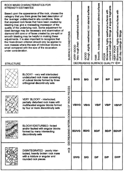
Figure 7: Characterization of rock masses on the basis of interlocking and joint alteration—from Hoek and Brown (1997).

Figure 8: Estimate of Geological Strength Index (GSI) based on geological descriptions—from Hoek and Brown (1997).
Spatial Variation and Randomness of Property Distribution
Material properties can be specified to adjust or to vary as a function of grid position. In fact, a different property can be assigned to every zone in a FLAC3D model, regardless of model size.
There are two commands avialable in FLAC3D to specfiy material properties. The first, zone property, allows multiple properties to be specified in a single command. This is convenient to completely specify properties in different regions, where that property does not vary within that region.
The second can only specify one property at a time, but has optional keywords that allow the property value to be automatically varied in space. This is the zone property-distribution command. Among the available keywords are add,
multiply, gradient, and vary, which can be used to provide fixed or linear variations of properties with position. For example, the following command provides a linear variation of cohesion in the \(x\)-direction:
zone property-distribution cohesion 1e6 gradient (-1e5,0,0)
An initial profile of a property can also be assigned via FISH.
With FLAC3D, it is also possible to study the influence of nonhomogeneity in a material. Any type of statistical property distribution can be introduced, as each element may have a unique property value. Two optional keywords are available to apply a random distribution of a selected property with the zone property-distribution command. The keyword
deviation-gaussian assumes a normal (Gaussian) distribution for the property, with a mean value, \(v\), and standard deviation, \(s\). The keyword deviation-uniform
assumes a uniform distribution with mean value, \(v\), and standard deviation, \(s\). Be careful to ensure that properties do not acquire negative values if \(s\) is large. As an example, the following command would give a mean friction angle of 40° with a standard deviation of 2. i.e. 95% of the friction values would be within ±10% of 40°:
zone property-distribution friction 40 deviation-gaussian 2
Use of the variation keywords in any command (not just for property variation) is defined in the topic Value Modifiers (add, multiply, gradient, & vary keywords).
| Was this helpful? ... | Itasca Software © 2024, Itasca | Updated: Dec 05, 2024 |
