
Zone
Orientation of Nodes and Faces within a Zone
A zone is a closed geometric domain, with nodes at the vertices and faces forming the surface of the zone. The relative orientation of the nodes and faces is shown in the figure below for the basic zone types: brick, wedge, pyramid, degenerate brick and tetrahedron (see zone create for full list). Each face has vertices; these vertices are also identified in the figure. Several FLAC3D and FISH commands (e.g., zone attach) refer to this orientation.
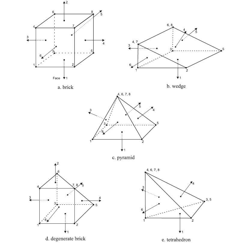
Figure 1: Zone geometry.
Condition Measure of Zones
A zone condition number is a measure of how badly deformed a zone is. Three measures are included, and the condition number is taken as the minimum of these three to characterize the worst case. The range of a zone condition number is between 0 and 1. The larger the zone number is, the better the zone geometry is.
The first measure is the smallest aspect ratio between the edges of each internal tetrahedron for a given zone. For all zone types, it is assumed that the ideal shape is the one for which all edges are equal in length, and angles between the edges are 90 degrees for a brick, 60 degrees and 90 degrees for a wedge or a degenerate brick, 60 degrees for a pyramid or a tetrahedron, so brick faces are squares, wedge faces are 3 squares and 2 equilateral triangles, pyramid faces are 1 square and 4 equilateral triangles, and tetrahedron faces are 4 equilateral triangles. For an ideal tetrahedron, the aspect ratio is 1. However, for the internal tetrahedrons composing zones with the ideal shapes, the smallest aspect ratio is \(1/ \sqrt 3\) for those internal tetrahedrons in an ideal brick or dbrick and \(1/ \sqrt 2\) for an ideal pyramid and wedge. Thus the result is required to be normalized to the range between 0 and 1 by multiplying a factor of \(\sqrt 3\) for bricks and dbricks, and \(\sqrt 2\) for pyramids and wedges.
The second measure is the volume ratio between the tetrahedron with the smallest volume and a tetrahedron with the “average” volume for a given zone. The average volume is defined as (zone volume) / (number of internal tetrahedrons). For wedge, tetrahedron, pyramid, and dbrick zone types with ideal shape, this measure gives 1. However, for an ideal brick, it gives 5/6. Thus the result is required to be normalized for bricks with a multiplication factor of 1.2.
The third measure is the orthogonality, which shows how “well” sides of the zones (for each face) are inclined relative to each other. If the test returns a value close to zero, it means that zone is most likely very elongated or badly deformed. For ideal brick, this minimum value is 1, but for other zone types with ideal shape, the minimum value is \(\sqrt 2\). Thus this measure has to be multiplied by \(1/ \sqrt 2\) for zones except bricks.
Zone Field Data Names
In FLAC3D, the FISH zone field data functions allow the user to make queries about the values of a model variable at arbitrary locations in space. This includes zone-based information as well as gridpoint-based information. The FISH functions in this section are state-based. Some of them set the particular data type (and the methods and properties used to get that data), while others retrieve the data once these values have been set.
By default, queries operate as quickly as possible for individual calls. If many (hundreds or more) points of data are to be queried, you can initialize the system to optimize multiple calls. This makes it unnecessary to calculate data more than once in a given zone or gridpoint. As an example, here is a FISH fragment that queries for the gridpoint-based value x-displacement at a single location in space:
zone.field.name = 'displacement-x'
local result = zone.field.get(vector(3.5,4.3,6.7))
Here is a FISH fragment that performs many queries on a line in space, on the zone-based values of horizontal stress:
array dataset(100)
zone.field.name = 'stress-xx'
zone.field.method.name = ’poly’ ; Use polynomial fit extrapolation
zone.field.init
loop ii (1,100)
   local xp = 5.0 + float(ii)/10.0
   dataset(ii) = zone.field.get(3.5,4.3,xp)
end_loop
zone.field.reset
The available zone field data names are described in the table below. Note that these are the same values available under zone history, for example.
Zone Field Data Names
| Name | Description |
|---|---|
| acceleration | acceleration magnitude at the gridpoint (only available if model configure dynamic has been specified) |
| acceleration-x | x-acceleration at the gridpoint (only available if model configure dynamic has been specified) |
| acceleration-y | y-acceleration at the gridpoint (only available if model configure dynamic has been specified) |
| acceleration-z | z-acceleration at the gridpoint (only available if model configure dynamic has been specified) |
| condition | a measure of how badly deformed a zone is (see discussion above) |
| density | the density of the zone |
| displacement | displacement magnitude at the gridpoint |
| displacement-x | x-displacement at the gridpoint |
| displacement-y | y-displacement at the gridpoint |
| displacement-z | z-displacement at the gridpoint |
| extra | extra variable value. The extra variable index used will default to 1 and can be changed with the zone.field.extra function. By default, the value will come from the grid point extra variables, but this can be specified using the zone.field.source function. By default, the value will be treated as a scalar floating point type, but this can be specified using the zone.field.type function. |
| pore-pressure | pore pressure in zone. By default, this will be the grid point pore pressure but the zone average pore pressure can be specified by using the zone.field.source function. |
| property | a property of the mechanical constitutive model of the zone. The property name must be specified using the zone.field.prop function. By default, it will be assumed the property is a floating point scalar but this can be specified using the zone.field.type function. |
| property-fluid | a property of the fluid constitutive model of the zone. The property name must be specified using the zone.field.prop function. By default, it will be assumed the property is a floating point scalar but this can be specified using the zone.field.type function. |
| property-thermal | a property of the thermal constitutive model of the zone. The property name must be specified using the zone.field.prop function. By default, it will be assumed the property is a floating point scalar but this can be specified using the zone.field.type function. |
| ratio-local | the local unbalanced force ratio at each gridpoint. Like all results, this can be changed to the logarithm of the value by using the zone.field.log function. |
| saturation | the saturation at the gridpoint (only available if model configure fluid has been specified) |
| strain-increment | the strain increment tensor of the zone determined by the current displacement field. Use the zone.field.quantity function to specify which scalar value to retrieve from the tensor. |
| strain-rate | the rate increment tensor of the zone determined by the current velocity field. Use the zone.field.quantity function to specify which scalar value to retrieve from the tensor. |
| stress | the stress tensor of the zone determined by the weighted average of the subzone stresses. Use the zone.field.quantity function to specify which scalar value to retrieve from the tensor. |
| stress-effective | the effective stress tensor of the zone determined by the weighted average of the subzone stresses minus the zone averaged pore pressure. Use the zone.field.quantity function to specify which scalar value to retrieve from the tensor. |
| stress-strength-ratio | the stress-strength ratio of the zone. Not all constitutive models support this calculation. If unsupported, the value returned will be 10. The value returned is generally held to a maximum of 10. |
| temperature | the temperature at the gridpoints. The zone.field.source function can be used to specify that zone-based temperature should be used instead. |
| timestep-dynamic | the local critical dynamic timestep of that particular gridpoint (only available if model configure dynamic has been specified) |
| unbalanced-force | the unbalanced force magnitude at the gridpoint |
| unbalanced-force-x | x-unbalanced force at the gridpoint |
| unbalanced-force-y | y-unbalanced force at the gridpoint |
| unbalanced-force-z | z-unbalanced force at the gridpoint |
| velocity | the velocity magnitude at the gridpoint |
| velocity-x | x-velocity at the gridpoint |
| velocity-y | y-velocity at the gridpoint |
| velocity-z | z-velocity at the gridpoint |
Zone Field Quantity Names
The field data names above may return a range of quantities. The options are listed in the following table. The definitions of the field data of a tensor (stress, strain increment, or strain rate) can be found in Stress/Strain Invariants.
| Quantity Name | Description |
|---|---|
| intermediate | intermediate principal stress or strain (increment/rate) |
| maximum | maximum (most positive) value of the principal stress or strain (increment/rate) |
| mean | mean value defined as the trace of the tensor divided by three |
| minimum | minimum (most negative) value of the principal stress or strain (increment/rate) |
| norm | norm of stress or strain (increment/rate) |
| octohedral | octahedral stress or strain (increment/rate) |
| shear-maximum | maximum shear stress or strain (increment/rate) |
| total-measure | distance from the origin to the tensor point in the principal space |
| volumetric | trace of the stress or strain (increment/rate) |
| von-mises | von Mises measure of the stress or strain (increment/rate) |
| xx | xx-component of the stress or strain (increment/rate) |
| xy | xy-component of the stress or strain (increment/rate) |
| xz | xz-component of the stress or strain (increment/rate) |
| yy | yy-component of the stress or strain (increment/rate) |
| yz | yz-component of the stress or strain (increment/rate) |
| zz | zz-component of the stress or strain (increment/rate) |
Below is a simple example:
zone.field.name = 'stress-xx'
zone.field.method.name = 'poly' ; Use polynomial fit extrapolation
global value1 = zone.field.get(10,0,-20) ; Return stress-xx
zone.field.quantity = 'von-mises' ; Reset the stress quantity to 'von-mises'
global value2 = zone.field.get(10,0,-20) ; Return stress-von-mises
or
zone.field.name = 'stress-xx'
zone.field.method.name = 'poly' ; Use polynomial fit extrapolation
global value1 = zone.field.get(10,0,-20) ; Return stress-xx
zone.field.name = 'stress-von-mises' ; Reset the filed name directly to 'stress-von-mises'
global value2 = zone.field.get(10,0,-20) ; Return stress-von-mises
Stress-Strength Ratio
The stress-strength ratio (SSR) is calculated in some constitutive models as a local indicator of the current stress state’s proximity to failure. Suppose the current effective minimum and maximum principal stresses are \(\sigma_1\) and \(\sigma_3\). The current Mohr circle is plotted in Figure 2. By keeping \(\sigma_3\) fixed, enlarge the Mohr circle so that it is tangent to the shear failure line; the new minimum effective principal stress is denoted by \(\sigma^{\prime}_1\), and the stress-strength ratio is defined as
It is self-evident that if the stress state is in shear failure, SSR = 1. The upper limit of SSR in FLAC3D is set to 10. If the current stress state is in tension failure, the SSR is set to 0. SSR can be plotted as a zone contour value if it is defined in the constitutive model.
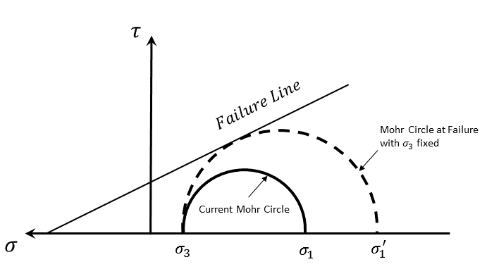
Figure 2: Schematic of stress-strength ratio.
| Was this helpful? ... | PFC 6.0 © 2019, Itasca | Updated: Nov 19, 2021 |