FLAC3D Theory and Background • Constitutive Models

Comparison between Mohr-Coulomb Model and Plastic-Hardening model

Note

To view this project in FLAC3D, use the menu command Help ? Examples…. Choose “ConstitutiveModels/ ComparisonPlasticHardening” and select “ComparisonPlasticHardening.f3dprj” to load. The project’s main data files are shown at the end of this example.

This example compares the behavior of the Plastic-Hardening (PH) model and Mohr-Coulomb (MC) model during the triaxial compression. Both models are used in a one-zone triaxial compression test with a constant cell pressure of 100 kPa. The strength parameters (including friction angle, dilation angle, and tension limit) are the same for both models. The $E_{50}$ stiffness of the PH model is used as Young’s modulus for the MC model and $E^{ref}_{ur}$ is assumed to be three times the value of $E^{ref}_{50}$. Material properties for this example are summarized in Table 1. Material parameters not listed in the table are default values.

Table 1: Model Properties for the Triaxial Compression Test

Parameters	PH	MC
$\phi$ (degrees)	30	30
$c$ (kPa)	0	0
$\psi$ (degrees)	10	10
$E^{ref}_{50}$ (kPa)	2e4
$E$ (kPa)		2e4
$\nu$	0.2	0.2
$E^{ref}_{ur}$ (kPa)	6e4
$m$	0.6
$R_f$	0.9
$p^{ref}$ (kPa)	100
$\sigma^{ini}_{1 \sim 3}$ (kPa)	-100

Figure 1 shows a plot deviatoric stress versus axial strain for both PH and MC models. It is easy to verify the following from the figure:

1. The ultimate failure deviatoric stresses (200 kPa) are the same for both models, as expected.
2. For the pre-failure curve, the PH and MC models are crossing at the half of the failure stress (100 kPa), which is consistent with the concept of $E_{50}$ stiffness.
3. The unloading stiffness in the MC model is the same as the loading stiffness ($E$ in the MC model, or $E_{50}$ in the PH model), while these stiffnesses are different in the PH model.

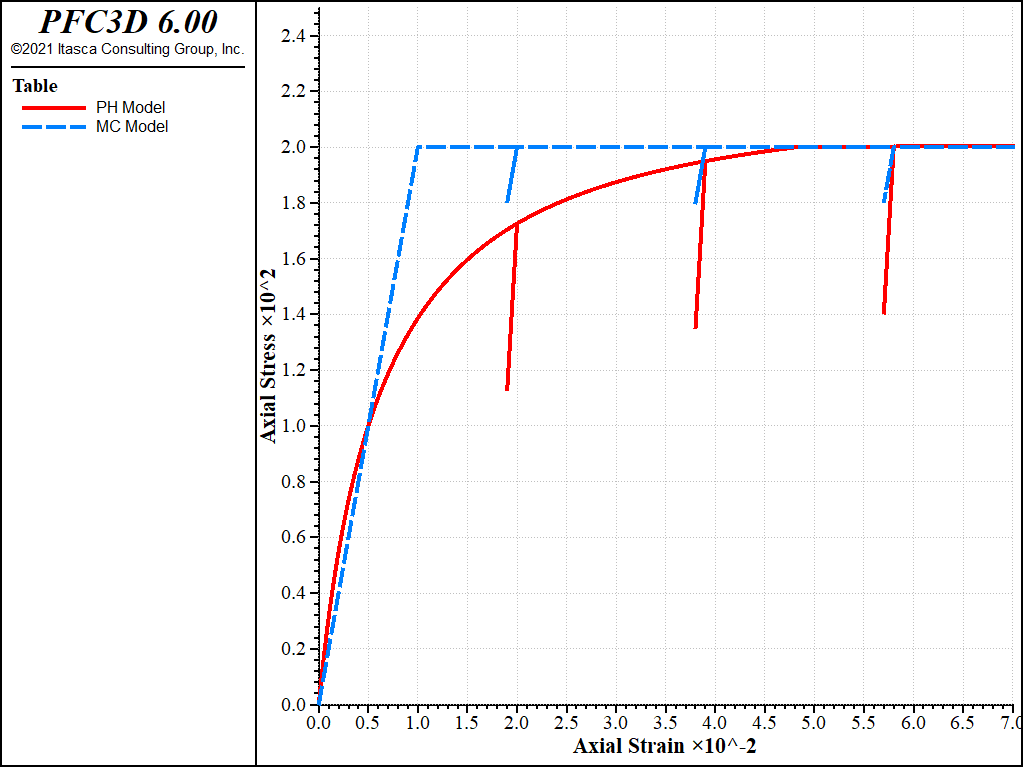
Figure 1: Comparison of PH and MC models for a triaxial compression test.

Data Files

TriaxialCompressionPlasticHardening.f3dat

model new
model largestrain off
;
zone create brick size 1 1 1
zone cmodel assign plastic-hardening
zone property stiffness-50-reference=2.0e4 stiffness-ur-reference=6.0e4 pressure-reference=100.0 exponent=0.6 poisson=0.2 failure-ratio=0.9
zone property friction=30.0 dilation=10.0 cohesion=0.0
zone property stress-1-effective=-100.0 stress-2-effective=-100.0 stress-3-effective=-100.0
;
zone gridpoint fix velocity-z
zone face apply stress-xx=-100.0 range union position-x 0 position-x 1
zone face apply stress-yy=-100.0 range union position-y 0 position-y 1
zone initialize stress xx -100.0 yy -100.0 zz -100.0
;
fish define hhhq_
    local zp_ = zone.head
    local gp_ = gp.find(8)
    global hhhq_ = zone.stress.xx(zp_) - zone.stress.zz(zp_)
    global hhha_ = -gp.disp.z(gp_)
end
history interval 10
fish history @hhhq_
fish history @hhha_
;
zone gridpoint initialize velocity-z -2e-6 range position-z 1
model step 10000
zone gridpoint initialize velocity-z  1e-6 range position-z 1
model step  1000
zone gridpoint initialize velocity-z -2e-6 range position-z 1
model step 10000
zone gridpoint initialize velocity-z  1e-6 range position-z 1
model step  1000
zone gridpoint initialize velocity-z -2e-6 range position-z 1
model step 10000
zone gridpoint initialize velocity-z  1e-6 range position-z 1
model step  1000
zone gridpoint initialize velocity-z -2e-6 range position-z 1
model step 20000
;
hist export  1 vs 2 table 'ph_qs_100'
table 'ph_qs_100' export 'ph_qs_100' truncate
;
model save 'ph100'

TriaxialCompressionMohrCoulomb.f3dat

model new
model largestrain off
;
zone create brick size 1 1 1
zone cmodel assign mohr-coulomb
zone property young=2.0e4 poisson=0.2 friction=30 dilation=10 cohesion=0.0
;
zone gridpoint fix velocity-z
zone face apply stress-xx=-100.0 range union position-x 0 position-x 1
zone face apply stress-yy=-100.0 range union position-y 0 position-y 1
zone initialize stress xx -100.0 yy -100.0 zz -100.0
;
fish define hhhq_
    local zp_ = zone.head
    local gp_ = gp.find(8)
    global hhhq_ = zone.stress.xx(zp_) - zone.stress.zz(zp_)
    global hhha_ = -gp.disp.z(gp_)
end
history interval 10
fish history @hhhq_
fish history @hhha_
;
zone gridpoint initialize velocity-z -2e-6 range position-z 1
model step 10000
zone gridpoint initialize velocity-z  1e-6 range position-z 1
model step  1000
zone gridpoint initialize velocity-z -2e-6 range position-z 1
model step 10000
zone gridpoint initialize velocity-z  1e-6 range position-z 1
model step  1000
zone gridpoint initialize velocity-z -2e-6 range position-z 1
model step 10000
zone gridpoint initialize velocity-z  1e-6 range position-z 1
model step  1000
zone gridpoint initialize velocity-z -2e-6 range position-z 1
model step 20000
;
hist export  1 vs 2 table 'mc_qs_100'
table 'mc_qs_100' export 'mc_qs_100' truncate
;
model save 'mc100'