Rough Strip Footing on a Cohesive Frictionless Material
Problem Statement
Note
To view this project in FLAC3D, use the menu command . Choose “VerificationProblems/PrandtlsWedge” and select “PrandtlsWedge.f3prj” to load. The data file used for hexahedral zones is shown at the end of this example. The remaining data files can be found in the project.
The prediction of collapse loads under steady plastic-flow conditions can be difficult for a numerical model to simulate accurately (Sloan and Randolph, 1982). As a two-dimensional example of a steady-flow problem, we consider the determination of the bearing capacity of a strip footing on a cohesive frictionless material (Tresca model). The value of the bearing capacity is obtained when steady plastic flow has developed underneath the footing, providing a measure of the ability of the code to model this condition.
The strip footing is located on an elasto-plastic material with the following properties:
shear modulus (\(G\)) 0.1 GPa bulk modulus (\(K\)) 0.2 GPa cohesion (\(c\)) 0.1 MPa friction angle (\(\phi\)) 0° dilation angle (\(\psi\)) 0°
Closed-Form Solution
The bearing capacity obtained as part of the solution to the “Prandtl’s wedge” problem is given by Terzaghi and Peck (1967) as
in which q is the average footing pressure at failure, and c is the cohesion of the material. The corresponding failure mechanism is illustrated in the figure below:

Figure 1: Prandtl mechanism for a strip footing.
FLAC3D Model
For this problem, half-symmetry and plane-strain conditions are assumed in the numerical simulation. The domain used for the analysis is sketched in the next figure, together with its dimensions.
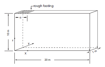
Figure 2: Domain for FLAC3D simulation—half symmetry.
A system of coordinate axes is selected as indicated in the figure. The area representing the strip footing has a half-width a, the far x-boundary is at a distance of 20 m from the y-axis of symmetry, and the far z-boundary is located 10 m below the footing. The thickness of the domain is selected as 1 m.
The boundary conditions applied to this domain are sketched in the next figure. The displacement of the rough footing is restricted in the y-direction, and a velocity is applied to the model in the negative z-direction to simulate the footing load. In the data file “PrandtlsWedge.f3dat”, the rightmost gridpoint of the footing is free in the x-direction. This condition can be justified because the physical constraint exactly at the edge is ambiguous and can be chosen arbitrarily. Releasing the constraint leads to a more uniform stress distribution under the footing, but does not affect the limit load.
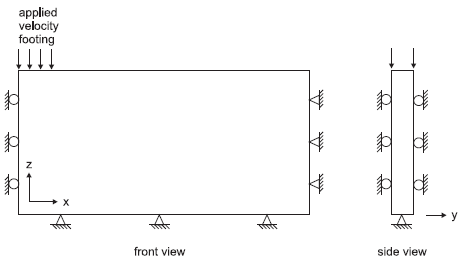
Figure 3: Boundary conditions for FLAC3D analysis—half symmetry.
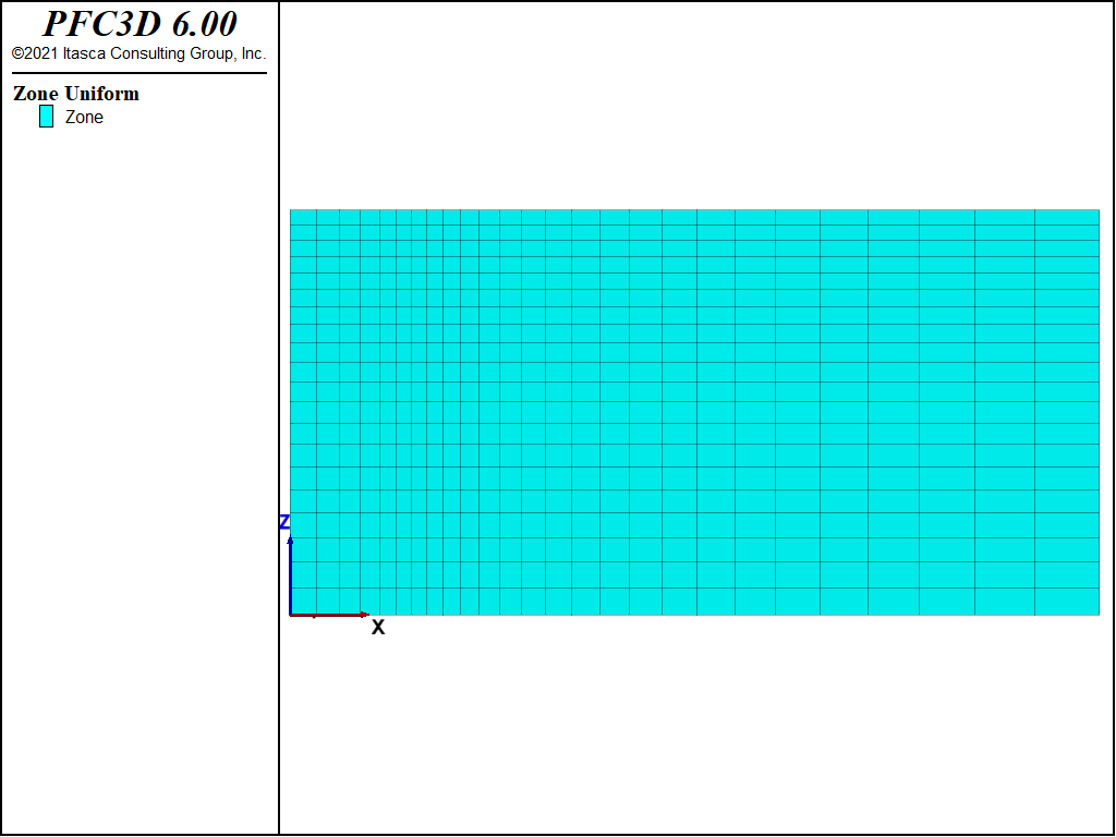
The domain is discretized into one layer of 520 zones organized in a graded pattern, as represented in Figure 4, with the grading arranged to increase definition (zone limits) in the areas of high strain gradient. The area representing the footing overlaps six zones, and a velocity of magnitude 0.5 × 10⁻⁵ m/step is applied at the contact nodes for a total of 25,000 calculation steps.
When a velocity is applied to gridpoints to simulate a footing load, the average footing pressure is found by assuming that the footing width is represented by a velocity that varies from the value at the last gridpoint to zero at the next gridpoint. The half-width, a, is then
where \(x_l\) is the \(x\)-location of the last applied gridpoint velocity, \(x_{l+1}\) is the \(x\)-location of the gridpoint adjacent to \(x_l\), and \(A\) accounts for the variation. If a linear variation is assumed, then \(A\) = 0.5, and \(a\) = 3.5 m for this problem. The effect of this assumption is discussed in Results And Discussion.
The FISH function load computes the numerical value of the normalized average footing pressure, \(p / c\).
Results and Discussion
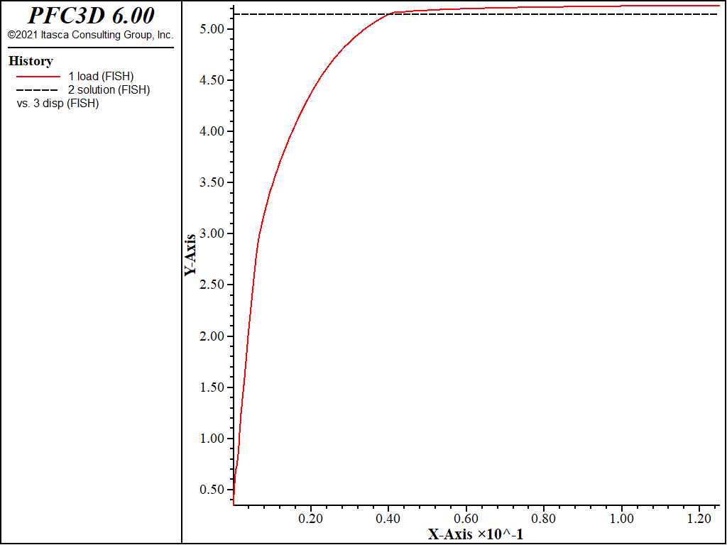
The load-displacement curve corresponding to the numerical simulation is presented in Figure 5, in which load is the normalized average footing pressure, \(p/c\), and disp is the magnitude of the normalized vertical displacement, \(u_z/a\), at the center of the footing. The numerical value of the bearing capacity, \(q\), is 523.0 kPa, and the relative error is 1.72% when compared to the analytical value of 514.2 kPa.
The apparent width of the footing is taken to be 3 m, plus half the zone width adjacent to the footing edge (because forces are exerted on the footing by this zone, it is assumed that the forces are divided equally between left and right gridpoints).
Note that the error in the bearing capacity is related to the indeterminacy in the apparent width of the footing. The mechanism illustrated in Figure 1 implies a velocity singularity at the ends of the footing. In a numerical simulation, this singularity is spread over the width of one zone. The apparent position of the velocity jump within that zone depends on the exact geometry of the velocity field that develops. In deriving \(q\), it is assumed that the jump occurs half a zone width from the end of the controlled boundary segment (\(A\) = 0.5 in Figure 2); note that if a variation factor of \(A\) = 0.63 is assumed, the error reduces to less than 0.1%. For finer grids, the indeterminacy in footing width decreases, and the match to the exact solution improves.
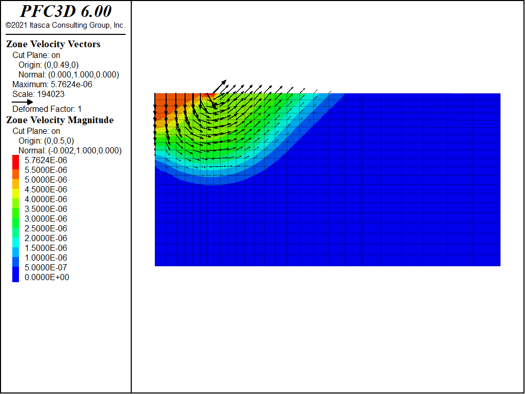
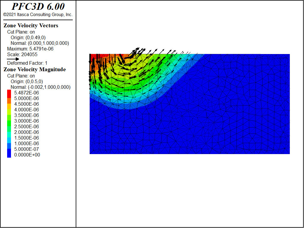
Velocity contours and velocity vectors at the end of the run are presented in Figure 6, showing good agreement with the mechanism in Figure 1.
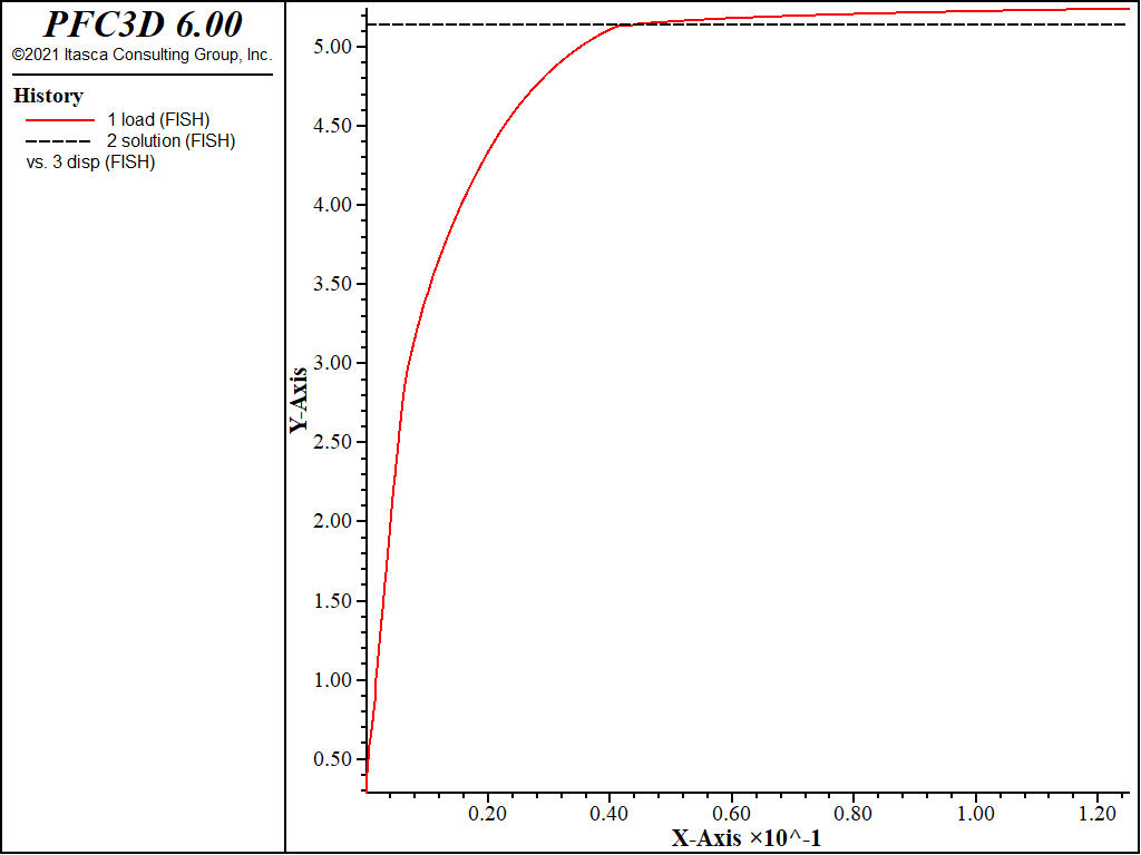
The same problem was run again using FLAC3D’s nodal mixed discretization (NMD) feature (file “nmd.f3dat”). For this model, an all-tet grid (file “nmd.f3grid”, which is generated using the file “create-tet-mesh.f3dat”) was used. The tet grid has gridpoints identical to the hex grid. With NMD, the numerical value of the bearing capacity, \(q\), is 524.1 kPa, and the relative error is 1.9% when compared to the analytical value of 514.2 kPa. As stated previously, the error in the bearing capacity is related to the indeterminacy in the apparent width of the footing. Figure 7 and Figure 8 show the NMD results, and correspond directly with Figure 5 and Figure 6 (results with an all-hex grid). As can be seen, the results are very similar.
References
Sloan, S. W., and M. F. Randolph. “Numerical Prediction of Collapse Loads Using Finite Element Methods,” Int. J. Num. & Analy. Methods in Geomech., 6, 47-76 (1982).
Terzaghi, K., and R. B. Peck. Soil Mechanics in Engineering Practice, 2nd Ed. New York: John Wiley and Sons (1967).
Data Files
;---------------------------------------------------------------------
; 2D rough strip footing on Tresca material (Prandtl's wedge problem)
; -associated plastic flow-
;---------------------------------------------------------------------
model new
model largestrain off
; Create zones
zone create brick size 6 1 20 point 1 (3.0,0.0,0.0) ...
                              point 3 (0.0,0.0,10.0) ...
                              ratio 0.9 1.0 0.97
zone create brick size 20 1 20 point 0 (3.0,0.0,0.0) ...
                               point 1 (20.0,0.0,0.0) ...
                               point 3 (3.0,0.0,10.0) ...
                               ratio 1.08 1.0 0.97
; Assign constitutive model and properties
zone cmodel assign mohr-coulomb
zone property bulk 2.e8 shear 1.e8 cohesion 1.e5
zone property friction 0. dilation 0. tension 1.e10
; Assign group name to footing surface
zone face group 'Footing' range position-x 0 3 position-z 10
; Boundary Conditions
zone face apply velocity-normal 0.0 range position-x 0
zone face apply velocity-normal 0.0 range union position-y 0 position-y 1
zone face apply velocity (0,0,0) range union position-x 20 position-z 0
zone gridpoint fix velocity (0,0,-0.5e-5) range position-x 0 3 position-z 10
zone gridpoint free velocity-x range position-x 3 position-z 10
; Call FISH function that monitors footing load
call 'footing-load'
@setup('Footing')
; Take some histories
fish history @load
fish history @solution
fish history @disp
model history mechanical ratio-local
; Cycle
model cycle 25000
; Save the model
model save 'pran'
return
⇐ Cylindrical Hole in an Infinite Hoek-Brown Medium | Smooth Circular Footing on an Associated Mohr-Coulomb Material ⇒
| Was this helpful? ... | PFC 6.0 © 2019, Itasca | Updated: Nov 19, 2021 |

