
Flat-Joint Model
The flat-joint model can be installed at both ball-ball and ball-facet contacts, and is referred to in commands and FISH by the name flatjoint.
Introduction
A flat-joint contact and its corresponding flat-jointed material are shown in Figure 1. The flat-joint contact model provides the macroscopic behavior of a finite-size, linear elastic, and either bonded or frictional interface that may sustain partial damage. A flat-jointed material mimics the microstructure of angular, interlocked grains that is similar to marble. The model formulation is given in this document. The initial two- and three-dimensional flat-joint models are described in [Potyondy2012a], [Potyondy2012b], and [Potyondy2013]. The present description defines both the 2D and 3D flat-joint models. The creation and laboratory testing of a flat-jointed material is described in the section “Example Materials 2: Flat-Jointed Material Example” in [Potyondy2017], which is provided in the material-modeling support package. Test problems that examine the behaviors of a single flat-jointed contact and an interlocked grain are provided in [Potyondy2016], which is included in the documentation of the material-modeling support package.
The formulation begins with a description of a flat-joint contact and its corresponding flat-jointed material, and is followed by a description of the flat-jointed interface. The activity-deletion criterion, force-displacement law, energy partitions, properties, methods, and callback events of the flat-joint contact model are then presented, followed by the stiffnesses required to determine a stable timestep. Expressions for element normal force and bending moment that are used in the force-displacement law are provided in the final subsection.
Behavior Summary
The behavior summary consists of a description of the flat-jointed material, followed by a description of the flat-jointed interface.
Flat-Jointed Material
A flat-joint contact and its corresponding flat-jointed material are shown in Figure 1. The flat-joint contact model provides the macroscopic behavior of a finite-size, linear elastic, and either bonded or frictional interface that may sustain partial damage. A flat-jointed material is defined in [Potyondy2017] as a granular assembly in which the flat-joint contact model exists at all grain-grain contacts with a gap less than or equal to the installation gap at the end of the material-finalization phase; all other grain-grain contacts as well as new grain-grain contacts that may form during subsequent motion are assigned the linear contact model. A flat-jointed material mimics a microstructure of angular, interlocked grains that is similar to marble.
Figure 1: Flat-joint contact (left) and flat-jointed material (right).
The flat-joint contact model provides the macroscopic behavior of a finite-size, linear elastic and either bonded or frictional interface that may sustain partial damage (see Figure 2). The interface is discretized into elements. Each element is either bonded or unbonded, and the breakage of each bonded element contributes partial damage to the interface. The behavior of a bonded element is linear elastic until the strength limit is exceeded and the bond breaks, making the element unbonded; the behavior of an unbonded element is linear elastic and frictional, with slip accommodated by imposing a Coulomb limit on the shear force. Each element carries a force and moment that obey the force-displacement law described below, while the force-displacement response of the flat-joint interface is an emergent behavior that includes evolving from a fully bonded state to a fully unbonded and frictional state.
Figure 2: Behavior and rheological components of the flat-joint model.
A flat-joint contact simulates the behavior of an interface between two notional surfaces, each of which is connected rigidly to a piece of a body. A flat-jointed material consists of bodies (balls, clumps, or walls) joined by flat-joint contacts such that the effective surface of each body is defined by the notional surfaces of its pieces, which interact at each flat-joint contact with the notional surface of the contacting piece. The notional surfaces are called faces, which are {lines in 2D; disks in 3D}.
The following description of a flat-jointed material applies to the case in which bodies are balls; however, the flat-joint model can be installed at both ball-ball and ball-facet contacts. We refer to the balls of a flat-jointed material as faced grains, each of which is depicted as a {circular in 2D; spherical in 3D} core and a number of skirted faces. The faced grains are created when the flat-joint model is installed at the ball-ball contacts of a packed ball assembly (see Figure 3). An interface exists between each set of adjoining faces and is discretized into elements, with each element being either bonded or unbonded. The breakage of each bonded element contributes partial damage to the interface, and each breakage event is denoted as a crack (see Figure 4)[1]. If the relative displacement at a flat-joint contact becomes larger than the flat-joint diameter, then the adjoining faces may be removed (because the contact may be deleted), making the associated balls locally {circular in 2D; spherical in 3D}. If these balls come back into contact, the behavior will be that of an interface between {circular in 2D; spherical in 3D} surfaces (if the linear contact model is assigned to the new contact).
Figure 3: Creation of faced grains showing packed ball assembly (left) and initial faced-grain assembly (right).
Figure 4: Partially damaged flat-jointed material showing faced grains with cracks colored red/blue for tensile/shear failure.
Flat-Jointed Interface
The interface of the flat-joint model remains centered on, and rotates with, the contact plane such that the interface coordinate system coincides with the contact-plane coordinate system. The interface gap \(\left(g,{\rm \; }g>0{\rm \; is\; open}\right)\) is expressed below in terms of the surface gap and the relative bend-rotation vector.[2] The relative motion of the notional surfaces varies over the interface, and is expressed by the symbols \(\stackrel{\frown}{\delta}\) and \(\stackrel{\frown}{\theta}\), which are related to the relative motion of the piece surfaces at the contact location:
where the relative displacement and rotation increments (\(\Delta {\pmb δ}\) and \(\Delta {\pmb θ}\)) are from Equation (12) in the “Contact Resolution” section. It is only the relative shear displacement (\(\Delta \stackrel{\frown}{{\pmb δ }}_{\mathbf s}\)) of the 3D model that varies over the interface (when the relative twist rotation is nonzero). Thus, the circumflex will be used only for this quantity. In the remainder of this section, we describe the kinematic variables and interface discretization, first for the 2D model and then for the 3D model.
The interface of the 2D flat-joint model is a rectangle of width \(2R\) and unit-thickness depth. The location of a point \(\mathbf{x}\) that lies on the interface is expressed by its relative position \({\mathbf r}={\mathbf x}-{\mathbf x}_{\mathbf c}\). The interface discretization (see Figure 5) is controlled by the number of equal-length elements in the radial direction (\(N_{r}\)). The area and centroid location of each element are denoted by \(A{\kern 1pt} ^{(e)}\) and \({\mathbf x}^{(e)}\), respectively. These quantities are given by
The quantities \(A{\kern 1pt} ^{(e)}\) and \(\rho ^{\left(e\right)}\) do not change during a simulation. They are set and stored during the first cycle after flat-joint installation.
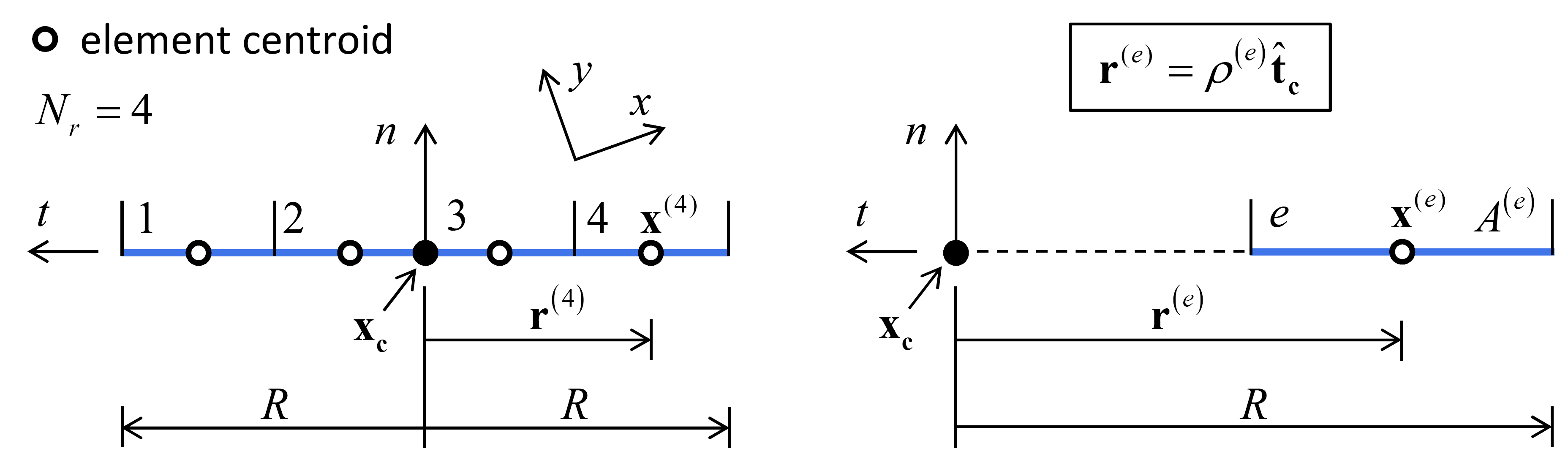
Figure 5: Interface discretization of the 2D flat-joint model showing element-numbering convention (left) and parameterization of a typical element (right).
The interface gap of the 2D flat-joint model (see Figure 6) is given by
where \(g_{s}\) is the surface gap and \({\pmb θ}_{\mathbf b}\) is the relative bend-rotation vector of Equation (12) in the “Contact Resolution” section. When expressed in the \(\gamma\) system, the interface gap varies only with \(\gamma\), and is related to \(g_{s}\) and \(\theta _{bk}\). The interface gap is not affected by the relative shear motion (which is a small-strain approximation).
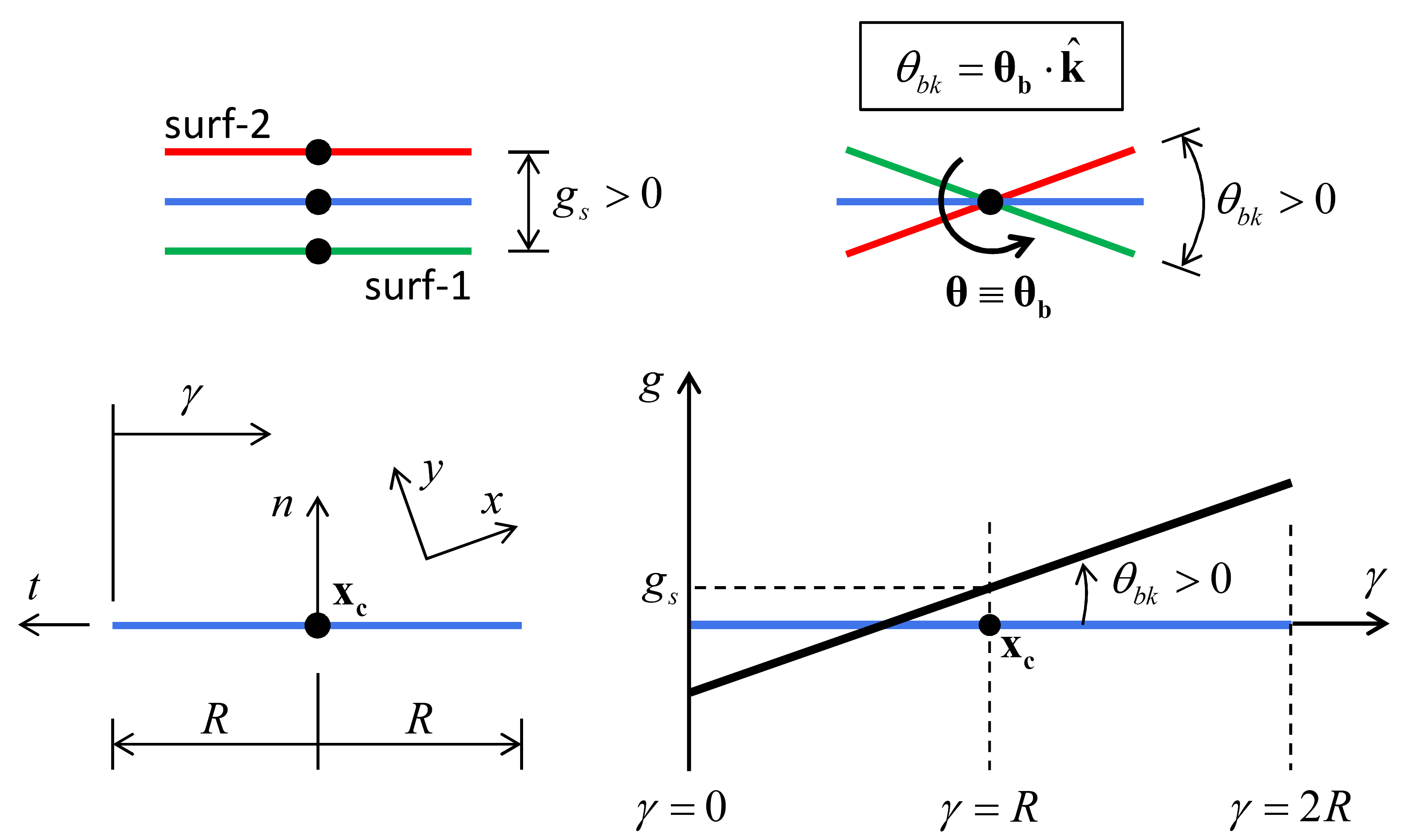
Figure 6: Interface gap of the 2D flat-joint model corresponding with motion at top of image.
For the 2D flat-joint model, the following components of the interface relative motion are tracked:
The interface of the 3D flat-joint model is a disk of diameter \(2R\). The location of a point \(x\) that lies on the interface is expressed by its relative position \({\mathbf r}={\mathbf x}-{\mathbf x}_{\mathbf c}\). The interface discretization (see Figure 7) is controlled by the number of elements in the radial (\(N_{r}\)) and circumferential (\(N_{\alpha }\)) directions. The area and centroid location of each element are denoted by \(A{\kern 1pt} ^{(e)}\) and \({\mathbf x}^{(e)}\), respectively. These quantities are given by
where the superscript \((e)\) notation has been dropped for the \(r\) and \(\alpha\) terms, which are given by
where \({\rm floor}\left(x\right)=\left\lfloor x\right\rfloor\) is the largest integer not greater than \(x\). The quantities \(A{\kern 1pt} ^{(e)}\), \(s^{\left(e\right)}\), and \(t^{\left(e\right)}\) do not change during a simulation. They are set and stored during the first cycle after flat-joint installation.
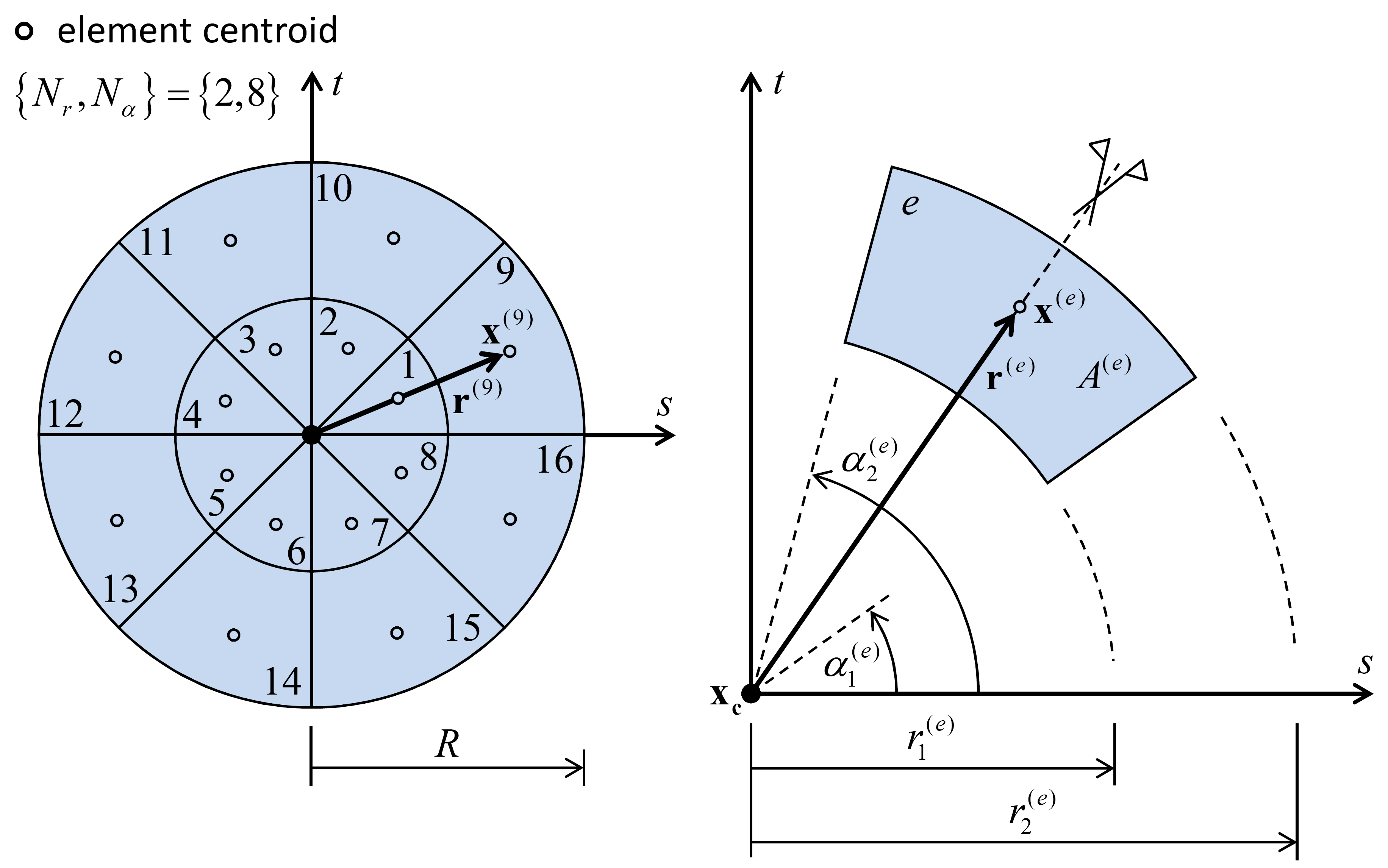
Figure 7: Interface discretization of the 3D flat-joint model showing element-numbering convention (left) and parameterization of a typical element (right).
There are two coordinate systems associated with the interface of the 3D flat-joint model (see Figure 8): the \(nst\) system, which coincides with the contact plane coordinate system, and the \(n\xi \eta\) system, which is dependent on the contact plane coordinate system as follows. The relative bend-rotation vector (\({\pmb θ }_{\mathbf b}\)) orients the \(n\xi \eta\) coordinate system such that \(\xi\) is aligned with \({\pmb θ }_{\mathbf b}\) (at an angle \(\beta _{s}\) from the positive \(s\) axis) and \(\hat{\mathbf n}_{\mathbf c} =\hat{\pmb \xi }\times \hat{\pmb \eta }\). The relative position of a point \(\pmb x\) that lies on the interface can be expressed in either coordinate system by the relations:
The mapping between these two coordinate systems of a vector \(\mathbf S\) that lies on the interface is given by the relations:
The interface gap of the 3D flat-joint model (see the next figure) is given by
where \(g_{s}\) is the surface gap and \({\pmb θ}_{\mathbf b}\) is the relative bend-rotation vector of Equation (12) in the “Contact Resolution” section. When expressed in the \(n\xi \eta\) system, the interface gap varies only with \(\eta\) and is related to \(g_{s}\) and \(\theta _{b\xi }\). The interface gap is not affected by the relative shear displacement or the relative twist rotation (which is a small-strain approximation). The interface gap is expressed in terms of \(s\), \(t\), and \(\beta_{s}\) (by substituting the mapping of Equation (8) into (9)):
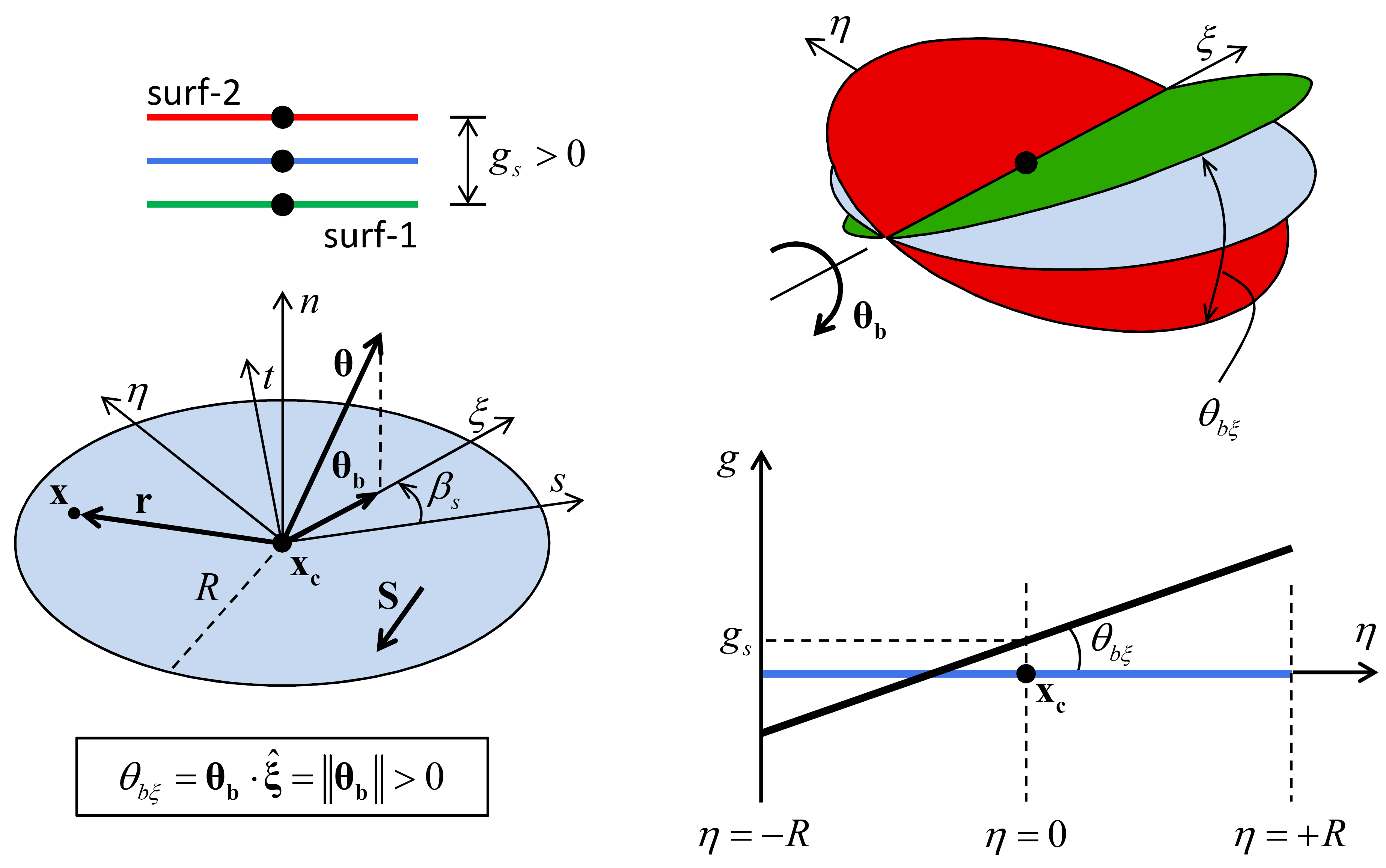
Figure 8: Interface gap of the 3D flat-joint model corresponding with motion at top of image.
For the 3D flat-joint model, the following components of the interface relative motion are tracked:
Activity-Deletion Criteria
A force may arise at a flat-joint element if it is either bonded or has a negative gap. The contact remains active until the distance between the centers of the notional surfaces is greater than the flat-joint diameter (\(\sqrt{g_{s} ^{2} +\left(\delta _{ss} \right)^{2} +\left(\delta _{st} \right)^{2} } >2R\)). Subsequently, the contact is deemed inactive and may be deleted. An inactive flat-joint contact may become active if the pieces overlap. In this case the notional surfaces are initialized.
Force Displacement Law
The force-displacement law for the flat-joint model updates the contact force and moment (\({\mathbf F}_{\mathbf c} =\tilde{\mathbf F}\) and \({\mathbf M}_{\mathbf c} =\tilde{\mathbf M}\)) that act at the contact location in an equal and opposite sense on the two pieces (see Figure 1 in the “Contacts Model Framework” topic). This is done by discretizing the interface into elements and providing a force-displacement law for each element so that the force-displacement response of the flat-joint interface is an emergent behavior. The force-displacement law for a flat-joint element is described in this section.
Each element carries a force and moment (\({\mathbf F}^{\left(e\right)}\) and \({\mathbf M}^{(e)}\)) that act at the element centroid in an equal and opposite sense on the notional surfaces. The element forces and moments produce a statically equivalent force and moment at the center of the interface (which coincides with the contact location—see Figure 9 and Figure 10) given by
where \({\mathbf r}^{\left(e\right)} ={\mathbf x}^{(e)} -{\mathbf x}_{c}\) is the relative position and \(x^{(e)}\) is the centroid location of element \((e)\). For the 2D model, Equation (12) becomes
by substituting \({\mathbf r}^{\left(e\right)}\) from Equation (2) into Equation (12) and expressing the element force in terms of its normal and shear components (defined below).
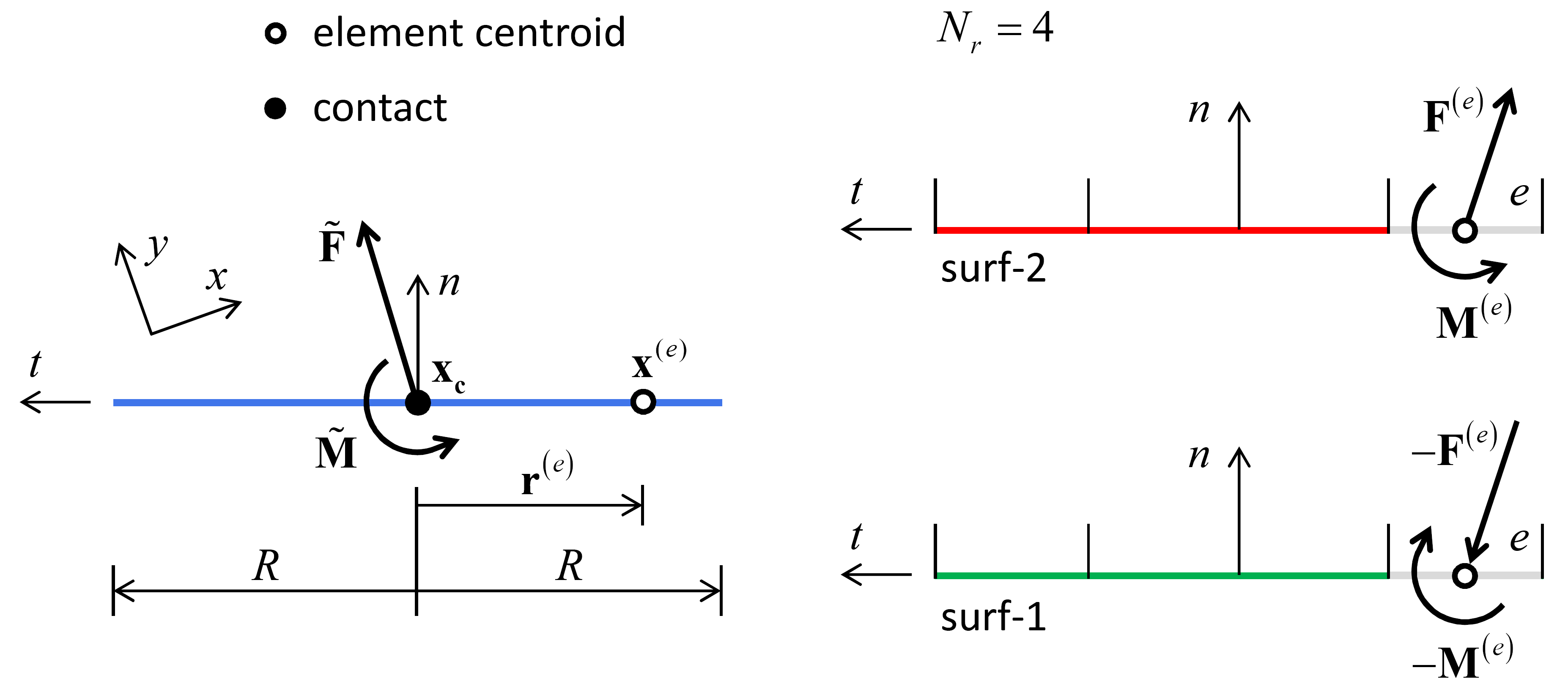
Figure 9: Force and moment acting on a typical 2D element (right) and its centroid relative position vector used to determine their contribution to force and moment at the center of the interface (left).
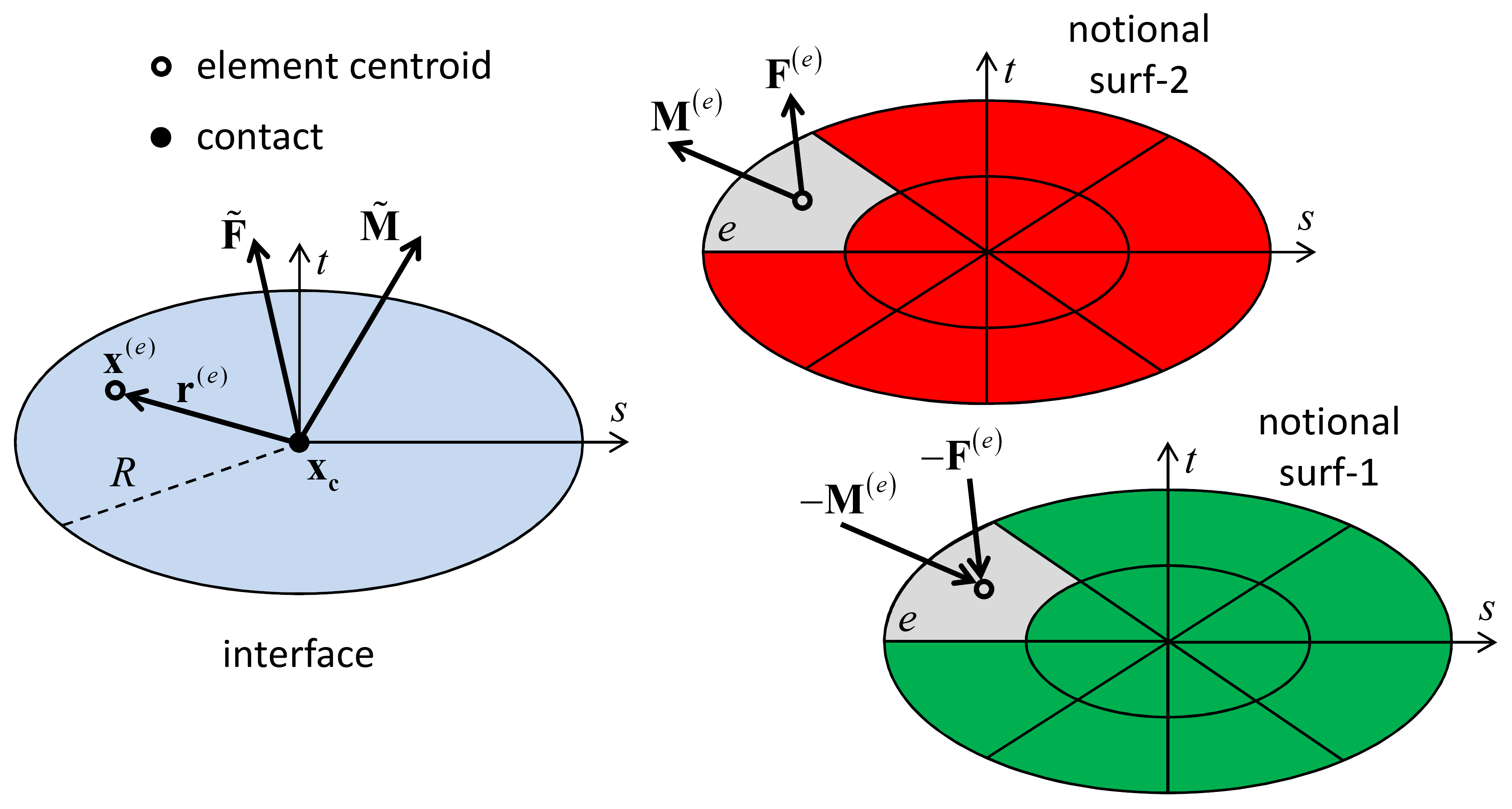
Figure 10: Force and moment acting on a typical 3D element (right) and its centroid relative position vector used to determine their contribution to force and moment at the center of the interface (left).
The force-displacement law for a flat-joint element updates the element force and moment (\({\mathbf F}^{\left(e\right)}\) and \({\mathbf M}^{(e)}\)), and may modify the element bond state (\(B^{(e)}\)). The element force is resolved into a normal and shear force, and the element moment is resolved into a twisting and bending moment:
where \(F_{n}^{(e)} >0\) is tension and \(M_{t}^{\left(e\right)} >0\) is shown in Figure 8 in the “Contact Resolution” section. The shear force and bending moment lie on the interface and are expressed in the interface coordinate systems:
For the 3D model, a simplifying assumption[3] gives \(M_{t}^{\left(e\right)} \equiv 0\). \(F_{n}^{\left(e\right)}\) and \({\mathbf M}_{\mathbf b}^{\left(e\right)}\) are updated by integrating the normal stress acting over the element, and \({\mathbf F}_{\mathbf s}^{(e)}\) is updated incrementally based on the effective portion of the relative shear-displacement increment at the element centroid.
The element normal and shear stresses are given by
where \(\sigma ^{(e)} >0\) is tension, and the stresses act at the element centroid. The interface normal stress \(\left(\sigma ,{\rm \; }\sigma >0{\rm \; is\; tension}\right)\) is given by
where \(k_{n}\) is the normal stiffness and \(g\) is the interface gap of {Equation (3) in 2D; Equation (10) in 3D}. The interface normal stress is proportional to the gap, and the unbonded region with a positive gap carries no load. A tensile load is carried only in a bonded region with a positive gap, and a compressive load is carried wherever the gap is negative (regardless of its bonding state). The gap and normal stress are continuous over the interface, and the gap may change sign within an element; however, the bonding is not continuous over the interface because each element is either bonded or unbonded (see below).
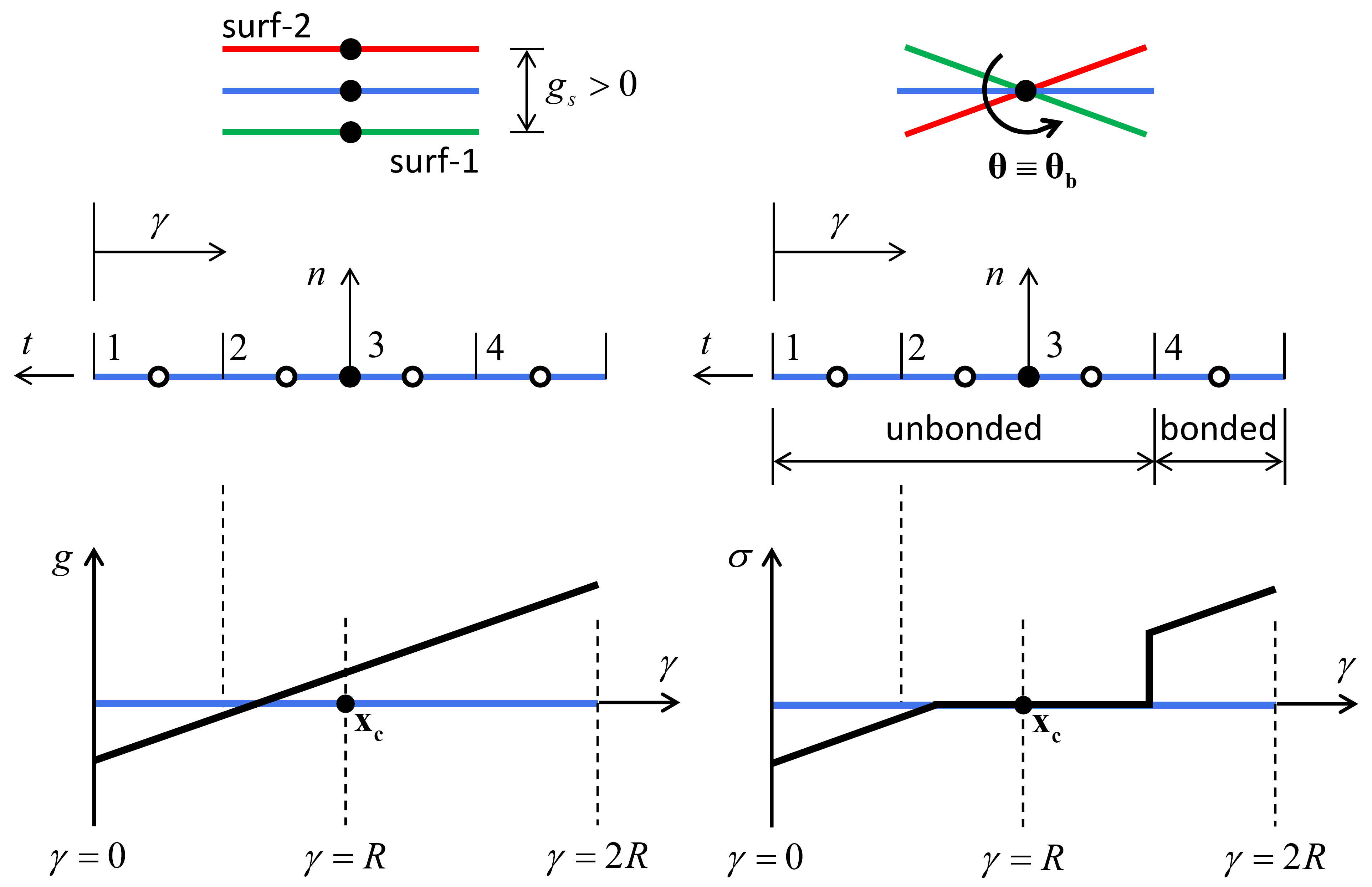
Figure 11: Variation of gap, normal stress, and bond state over a four-element, 2D flat-joint model corresponding with motion at top of image.
When the flat-joint model is installed at a contact, the following quantities are initialized:
When the first cycle occurs after the flat-joint model is installed at a contact, the following properties are fixed:
and initialized:
The first condition establishes the initial location and orientation of the notional surfaces relative to the pieces. The initial surface gap (\(g_{o}\), \(g_{o} >0\) is open) is the distance between the finite-size notional surfaces measured along the dotted line in Figure 2. The surface gap \((g_{s} =g_{o} +\sum \Delta \delta _{n}\), \(g_{s} >0\) is open) is the cumulative relative normal displacement of the piece surfaces.
The force-displacement law for a flat-joint element consists of the following steps (see Figure 12 and Figure 13).
Update \(F_{n}^{(e)}\):
(21)\[F_{n}^{(e)} =\int _{e}\sigma dA\]where \(\sigma\) is the interface normal stress of Equation (17), and the integration is performed over element (\(e\)). Analytical expressions for this integral (given in the section “Expressions for Element Normal Force and Bending Moment” below) are used to update \(F_{n}^{(e)}\), which in turn, is used to update \(\sigma ^{(e)} ={F_{n}^{\left(e\right)} \mathord{\left/ {\vphantom {F_{n}^{\left(e\right)} A^{\left(e\right)} }} \right. } A^{\left(e\right)} }\). If the element is bonded and the tensile-strength limit is exceeded (\(\sigma ^{(e)} >\sigma _{c}\)), then break the bond in tension \(\left(B^{(e)} =1,\; \; \left\{F_{n}^{(e)} ,F_{ss}^{(e)} ,F_{st}^{(e)} \right\}=0\right)\), trigger the bond-break callback event, and skip the next step. If the element is unbonded and \(\sigma ^{(e)} \ge 0\), then set the element shear force to zero \(\left(\left\{F_{ss}^{(e)} ,F_{st}^{(e)} \right\}=0\right)\) and skip the next step.
Update \(F_{s}^{(e)}\) as follows. Compute a trial element shear force:
(22)\[\begin{split}\begin{array}{ll} {\mathbf F}_{\textbf s}^{(e)'} = {\textbf F}_{\textbf s}^{(e)} -k_{s} A^{(e)} \Delta \stackrel{\frown}{\pmb δ}_{s}^{(e)'} & \left[ F_{ss}^{(e)'} =F_{ss}^{(e)} -k_{s} A^{(e)} \Delta \stackrel{\frown}{\delta }_{ss}^{(e)'} ,\; \; F_{st}^{(e)'} =F_{st}^{(e)} -k_{s} A^{(e)} \Delta \stackrel{\frown}{\delta }_{st}^{(e)'} \right] \\[5mm] {\rm with} \ \ \Delta\stackrel{\frown}{\pmb δ}_{\textbf s}^{(e)'} = \alpha\Delta\stackrel{\frown}{\pmb δ}_{\textbf s}^{(e)} & \left[\Delta \stackrel{\frown}{\delta }_{ss}^{(e)'} =\alpha \Delta \stackrel{\frown}{\delta }_{ss}^{(e)} ,\; \; \Delta \stackrel{\frown}{\delta }_{st}^{(e)'} =\alpha \Delta \stackrel{\frown}{\delta }_{st}^{(e)} \right] \end{array} \\[3mm] \alpha =\left\{\begin{array}{l} {\frac{g_{1}^{(e)} }{g_{1}^{(e)} -g_{0}^{(e)} } ,\qquad {\rm unbonded\; and\; }g_{0}^{(e)} >0{\rm \; and\; }g_{1}^{(e)} <0} \\[3mm] {\qquad 1,\qquad {\rm otherwise}} \end{array}\right.\end{split}\]where \(\Delta \stackrel{\frown}{\pmb δ }_{\mathbf s}^{(e)'}\) is the effective portion of the relative shear-displacement increment at the element centroid. If the element is bonded, then the entire increment is effective; if the element is not bonded, then only the portion of the increment that occurs while \(g^{\left(e\right)} <0\) is effective; \(\Delta \stackrel{\frown}{\pmb δ }_{\mathbf s}^{(e)}\) is \(\Delta \stackrel{\frown}{\pmb δ }_{\mathbf s}\) of Equation (1) evaluated at the element centroid and \(g^{\left(e\right)}\) at the beginning and end of the timestep is denoted by \(g_{0}^{(e)}\) and \(g_{1}^{(e)}\), respectively. The trial element shear stress:
(23)\[\tau ^{(e)'} ={\left\| {\mathbf F}_{\mathbf s}^{(e)'} \right\| \mathord{\left/ {\vphantom {\left\| {\mathbf F}_{\mathbf s}^{(e)'} \right\| A^{(e)} }} \right. } A^{(e)} } .\]The procedure now differs based on the bond state as follows.
- Unbonded. The shear strength \(\tau _{c}^{(e)} = c_r-\mu \sigma ^{(e)}\). If \(\left|\tau ^{(e)'} \right|\le \tau _{c}^{(e)}\), then \({\mathbf F}_{\mathbf s}^{(e)} ={\mathbf F}_{\mathbf s}^{(e)'}\); otherwise, enforce the shear-strength limit \(\left({\mathbf F}_{\mathbf s}^{(e)} =\tau _{c}^{(e)} A^{(e)} \left({{\mathbf F}_{\mathbf s}^{(e)'} \mathord{\left/ {\vphantom {{\mathbf F}_{\mathbf s}^{(e)'} \left\| {\mathbf F}_{\mathbf s}^{(e)'} \right\| }} \right. } \left\| {\mathbf F}_{\mathbf s}^{(e)'} \right\| } \right)\right)\), which implies that slip has occurred and the slip energy is updated via Equation (28). If the slip state has changed, then trigger the slip-change callback event.
- Bonded. The shear strength \(\tau _{c}^{\left(e\right)} = c-\sigma ^{\left(e\right)} \tan \phi\). If \(\left|\tau ^{(e)'} \right|\le \tau _{c}^{(e)}\), then \({\mathbf F}_{\mathbf s}^{(e)} ={\mathbf F}_{\mathbf s}^{(e)'}\); otherwise, the shear-strength limit has been exceeded. Break the bond in shear (by setting \(B^{(e)} =2\), reevaluating \(F_{n}^{\left(e\right)}\) as in step 1 and triggering the bond-break callback event). If \(M_r = 0\) (shear drop to zero), then set \(\left\{F_{ss}^{(e)} ,F_{st}^{(e)} \right\}=0\). If \(M_r = 1\) (shear drop to residual), then set \({\mathbf F}_{\mathbf s}^{(e)} = (c_r-\mu \sigma ^{(e)}) A^{(e)} \left({{\mathbf F}_{\mathbf s}^{(e)'} \mathord{\left/ {\vphantom {{\mathbf F}_{\mathbf s}^{(e)'} \left\| {\mathbf F}_{\mathbf s}^{(e)'} \right\| }} \right. } \left\| {\mathbf F}_{\mathbf s}^{(e)'} \right\| } \right)\).
Update \(M_{b}^{(e)}\):
(24)\[M_{b}^{(e)} =-\int _{e}r\sigma dA\]where \(\sigma\) is the interface normal stress of Equation (17), \(r\) is the moment arm with respect to the element centroid, and the integration is performed over element (\(e\)). Analytical expressions for this integral (given in the section “Expressions for Element Normal Force and Bending Moment” below) are used to update \(M_{b}^{(e)}\).
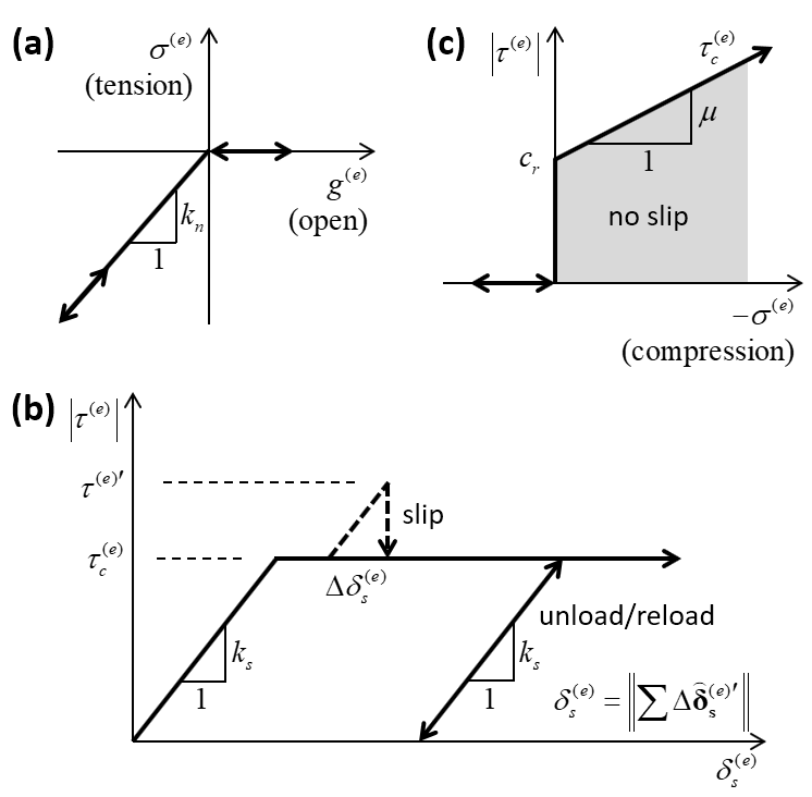
Figure 12: Force-displacement law for an unbonded flat-joint element: (a) normal stress versus element gap; (b) shear stress versus relative shear displacement; and (c) slip envelope.
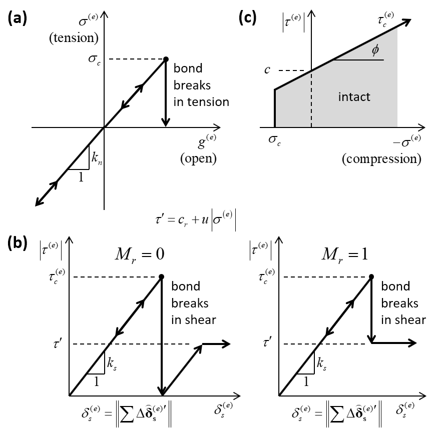
Figure 13: Force-displacement law for a bonded flat-joint element: (a) normal stress versus element gap; (b) shear stress versus relative shear displacement; and (c) failure envelope.
Energy Partitions
The flat-joint model provides two energy partitions:
- strain energy, \(E_{k}\), stored in the springs; and
- slip energy, \(E_{\mu}\), defined as the total energy dissipated by frictional slip.
The strain energy in the flat joint is obtained by summing the strain energy in each element:
The strain energy in each element is updated after the force-displacement law:
where \(I^{\left(e\right)}\) is the moment of inertia of the element cross-section (about the line passing through \({\mathbf x}^{\left(e\right)}\) and in the direction of \({\pmb θ }_{\mathbf b}\)), \(J^{\left(e\right)}\) is the polar moment of inertia of the element cross-section (about the line through \({\mathbf x}^{\left(e\right)}\) and in the direction of \(\hat{\mathbf n}_{c}\)), \(\bar{r}\) is the element half-length, and \(r_{e}\) is the element effective radius. The integrals in Equation (26) are {evaluated exactly in 2D; and approximated in 3D} (by assuming that the element is a disk with an area equal to that of the element).
The slip energy in the flat joint is obtained by summing the slip energy in each element:
The slip energy in each element is updated during the force-displacement law whenever the shear-strength limit has been exceeded via:
where the quantities are defined in the “Force Displacement Law” section.
| Keyword | Symbol | Description | Range | Accumulated |
|---|---|---|---|---|
energy‑strain |
\(E_{k}\) | strain energy | \([0.0,+\infty)\) | NO |
energy‑slip |
\(E_{\mu}\) | total energy dissipated by slip | \([0.0,+\infty)\) | YES |
Properties
The properties defined by the flat-joint contact model are listed in the table below as a concise reference; see the “Contact Properties” section for a description of the information in the table columns.
| Keyword | Symbol | Description | Type | Range | Default | Modifiable | Inheritable |
|---|---|---|---|---|---|---|---|
flatjoint |
Model name | ||||||
fj_nr |
\(N_r\) | Number of elements in radial direc. (total number of elements in 2D) | INT | [1, ∞) | 2 | NO [1] | NO |
fj_nal (3D) |
\(N_\alpha\) | Number of elements in circumferential direc. | INT | [3, ∞) | 4 | NO [1] | NO |
fj_rmul |
\(\lambda\) | Radius multiplier | FLT | (0.0, ∞) | 1.0 | NO [1] | NO |
fj_gap0 |
\(g_0\) | Initial surface gap | FLT | [0.0, ∞) | 0.0 | NO[1] \((\{g_o > 0 \} \Rightarrow \{\forall e: B^{(e)} = 0 \} )\) | NO |
fj_kn |
\(k_n\) | Normal stiffness [stress/disp.] | FLT | [0.0, ∞) | 0.0 | YES | NO |
fj_ks |
\(k_s\) | Shear stiffness [stress/disp.] | FLT | [0.0, ∞) | 0.0 | YES | NO |
fj_fric |
\(\mu\) | Friction coefficient | FLT | [0.0, ∞) | 0.0 | YES | NO |
fj_ten |
\(\sigma_c\) | Tensile strength [stress] | FLT | [0.0, ∞) | 0.0 | YES | NO |
fj_coh |
\(c\) | Cohesion [stress] | FLT | [0.0, ∞) | 0.0 | YES | NO |
fj_cohres |
\(c_r\) | Residual cohesion [stress] | FLT | [0.0, ∞) | 0.0 | YES | NO |
fj_fa |
\(\phi\) | Friction angle [degrees] | FLT | [0.0, 90.0) | 0.0 | YES | NO |
fj_resmode |
\(M_r\) | Shear-drop residual mode \(\left\{\begin{array}{l} {0, {\rm shear \;drop \;to \;zero}} \\ {1, {\rm shear \;drop \;to \;residual}} \end{array} \right\}\) | INT | {0,1} | 0 | YES | NO |
fj_elem |
\(e\) | Element ( \(e\) ) — accesses element-based data (element numbering in Figure 5 and Figure 16) | INT | [1, \(N_r N_\alpha\)] | 1 | YES | NO |
fj_emod |
\(E^*\) | Effective modulus | FLT | [0.0, ∞) | 0.0 | NO | NO |
fj_kratio |
\(\kappa^*\) | Normal-to-shear stiffness ratio, \(\kappa^* \equiv k_n / k_s\) | FLT | [0.0, ∞) | 0.0 | NO [2] | NO |
fj_slip |
\(s^{(e)}\) | Slip state of element \((e)\) \(\left\{ \begin{array}{rl} {\rm true} ,& {\rm slipping} \\ {\rm false} ,& {\rm not \;slipping} \end{array} \right\}\) | BOOL | {true,false} | false | NO | NO |
fj_state |
\(B^{(e)}\) | Bond state of element \((e)\) \(\left\{\begin{array}{l} {0, {\rm unbonded}} \\ {1, {\rm unbonded \;\& \;broke \;in \;tension}} \\ {2, {\rm unbonded \;\& \;broke \;in \;shear}} \\ {3, {\rm bonded}} \end{array} \right\}\) | INT | {0,1,2,3} | 0 | NO | NO |
fj_radius |
\(R\) | Flat-joint radius | FLT | (0, ∞) | NA | NO (set via \(\lambda\)) | NO |
fj_gap |
\(g_s\) | Surface gap | FLT | \(\mathbb{R}\) | \(g_o\) | NO | NO |
fj_relbr |
\({\pmb θ}_{\mathbf b}\) | Relative bend-rotation \((\theta_{bs} , \theta_{bt})\) (2D model: \(\theta_{bk} = -\theta_{bs} , \theta_{bt} \equiv 0\)) | VEC2 | NA | \(\textbf 0\) | NO | NO |
fj_cen |
\(\mathbf{x}^{(e)}\) | Centroid location of element \((e)\) | VEC | NA | NA | NO | NO |
fj_area |
\(A^{(e)}\) | Area of element \((e)\) | FLT | (0, ∞) | NA | NO | NO |
fj_egap |
\(g^{(e)}\) | Gap at centroid of element \((e)\) | FLT | \(\mathbb{R}\) | NA | NO | NO |
fj_shear |
\(\tau_c^{(e)}\) | Shear strength [stress] at centroid of element \((e)\) | FLT | [0.0, ∞) | 0.0 | NO (set via \(c\) and \(\sigma_c\)) | NO |
fj_sigma |
\(\sigma^{(e)}\) | Normal stress at centroid of element \((e)\) | FLT | \(\mathbb{R}\) | NA | NO | NO |
fj_tau |
\(\tau^{(e)}\) | Shear stress at centroid of element \((e)\) | FLT | [0.0, ∞) | NA | NO | NO |
fj_force |
\(\tilde{{\mathbf F}}\) | Interface force | VEC | NA | \(\textbf 0\) | NO | NO |
fj_moment |
\(\tilde{{\mathbf M}}\) | Interface moment | VEC | NA | \(\textbf 0\) | NO | NO |
fj_track |
Tracking state for use when plotting contacts with the specific numeric value | BOOL | {true,false} | false | YES | NO | |
fj_mtype |
Initial microstructural type \(\left\{\begin{array}{l} {1, {\rm bonded}} \\ {2, {\rm gapped}} \\ {3, {\rm slit}} \\ {4, {\rm undefined}} \end{array} \right\}\) | INT | {1,2,3,4} | NA | NO | NO | |
user_area |
\(A\) | Constant area [length*length] | FLT | \((0.0,+\infty)\) | 0.0 | YES | NO |
[1] Specify before cycling; cannot modify thereafter.
[2] If either the normal or shear stiffness is zero, then \(\kappa^*\) is zero.
Methods
| Method | Argument | Symbol | Type | Range | Default | Description |
|---|---|---|---|---|---|---|
| area | Set user_area to the area | |||||
| deformability | Set deformability | |||||
| emod | \(E^*\) | FLT | [0.0,+ ∞) | NA | Effective modulus | |
| kratio | \(\kappa^* \equiv k_n / k_s\) | FLT | [0.0,+ ∞) | NA | Normal-to-shear stiffness ratio | |
| initialize | Initialize the forces and moment. | |||||
| force | VEC | Total local force | ||||
| Moment | VEC | Total local moment | ||||
| bond | Bond element ( e ) or all elements | |||||
| element | Element number ( e ) [1] | |||||
| gap | \(G\) | VEC2 | \(\mathbb{R}^2\) | \((-\infty,0]\) | Gap interval | |
| unbond | Unbond element ( e ) or all elements. | |||||
| element | Element number ( e ) [1] | |||||
| gap | \(G\) | VEC2 | \(\mathbb{R}^2\) | \((-\infty,0]\) | Gap interval | |
[1] Element numbering is shown in figures above.
Area
Set the user_area property via the current contact area. This operation means that the contact area stays constant and is fixed independent of changes to the piece sizes/geometries. In order for the stiffnesses to be recomputed accounting for this area, one should subsequently call the deformabilty method.
Deformability
The deformability provided by the flat-joint interface can be specified with the deformability method which sets:
The first term in this expression is obtained by equating the normal stiffness to the axial stiffness of the volume of material shown in Figure 6 of the “Linear Model” description.
The deformability of a homogeneous, isotropic, and well-connected granular assembly experiencing small-strain deformation can be fit by an isotropic material model, which is described by the elastic constants of Young’s modulus (\(E\)) and Poisson’s ratio (\(\nu\)). \(E\) and \(\nu\) are emergent properties that can be related to the effective modulus (\(E^{*}\)) and the normal-to-shear stiffness ratio (\(\kappa ^{*} \equiv {k_{n} \mathord{\left/ {\vphantom {k_{n} k_{s} }} \right. } k_{s} }\)) at the contact as follows: \(E\) is related to \(E^{*}\) with \(E\) increasing as \(E^{*}\) increases, and \(\nu\) is related to \(\kappa ^{*}\) with \(\nu\) increasing up to a limiting positive value as \(\kappa ^{*}\) increases. These relationships are obtained by specifying \(E^{*}\) and \(\kappa ^{*}\) as the arguments of the deformability method.
Initialize
Initialize the local force and moment presuming all elements are bonded. This can be useful when inserting a flat-joint model in a preexisting contact in a system that has been cycled to equilibrium. The gaps of each element are set to provide the desired force. A separate moment is stored and added to each bonded element to produce the desired moment.
Bond
Bond element (\(e\)) if the contact gap between the pieces is within the bonding-gap interval. If no gap is specified, then the element is bonded if the pieces overlap. A single value can be specified with the gap keyword corresponding to the maximum gap. If the element number (\(e\)) is not specified, then all elements are bonded. Only elements with a zero gap over their entire surface can be bonded. If an element becomes bonded, then the element bond state becomes bonded (\(B^{\left(e\right)} =3\)). The element force and moment are unaffected and will be updated during the next cycle. One can ensure the existence of contacts between all pieces with a contact gap less than a specified bonding gap (\(g_{b}\)) by specifying \(g_{b}\) with the proximity in the contact cmat default command of the Contact Model Assignment Table (CMAT).
Unbond
Unbond element (\(e\)) if the contact gap between the pieces is within the bonding-gap interval. If no gap is specified, then the element is unbonded if the pieces overlap. A single value can be specified with the gap keyword corresponding to the maximum gap. If an element number (\(e\)) is not specified, then unbond all elements. If the element becomes unbonded, then the element bond state becomes unbonded (\(B^{\left(e\right)} =0\)). The element force and moment are unaffected and will be updated during the next cycle.
Callback Events
| Event | Array Slot | Value Type | Range | Description |
|---|---|---|---|---|
| contact_activated | Contact has become active | |||
| 1 | C_PNT | N/A | Contact address | |
| slip_change | Slip state of element ( e ) has changed. | |||
| 1 | C_PNT | NA | Contact address | |
| 2 | Element number ( e ) [1] | |||
| 3 | INT | {0,1} | Slip change mode \(\;\;\;\;\;\;\begin{cases} \mbox{0: slip has initiated} \\ \mbox{1: slip has ended} \end{cases}\) | |
| bond_break | Bond of element ( e ) has broken. | |||
| 1 | C_PNT | NA | Contact address | |
| 2 | Element number ( e ) [1] | |||
| 3 | INT | {1,2} | Break mode \(\;\;\;\;\;\;\begin{cases} \mbox{1: broke in tension} \\ \mbox{2: broke in shear} \end{cases}\) | |
| 4 | FLT | [0.0,+ ∞) | Strain energy at onset of failure | |
| broken | All bonds are broken. | |||
| 1 | C_PNT | NA | Contact address | |
[1] Element numbering is shown in figures above.
Stiffnesses for Timestep Estimation Scheme
Expressions for Element Normal Force and Bending Moment
Analytical expressions for the element normal force and bending moment (\(F_{n}^{\left(e\right)}\) and \(M_{b}^{(e)}\)) are presented here. These expressions are obtained by integrating the interface normal stress over the element. The element normal force and bending moment satisfy:
where \(\sigma\) is the interface normal stress of Equation (17), \(r\) is the moment arm with respect to the element centroid, and the integration is performed over element (\(e\)). These integrals are {evaluated exactly in 2D; and approximated in 3D}.
For the 2D model, the integrals are evaluated exactly as follows. The gap across the element (see Figure 14) is given by
where \(g_{a}^{\left(e\right)}\) and \(g_{b}^{\left(e\right)}\) are the values of the gap at the element ends (obtained by evaluating Equation (3) at these locations) and \(\bar{r}^{\left(e\right)}\) is the element half-length.
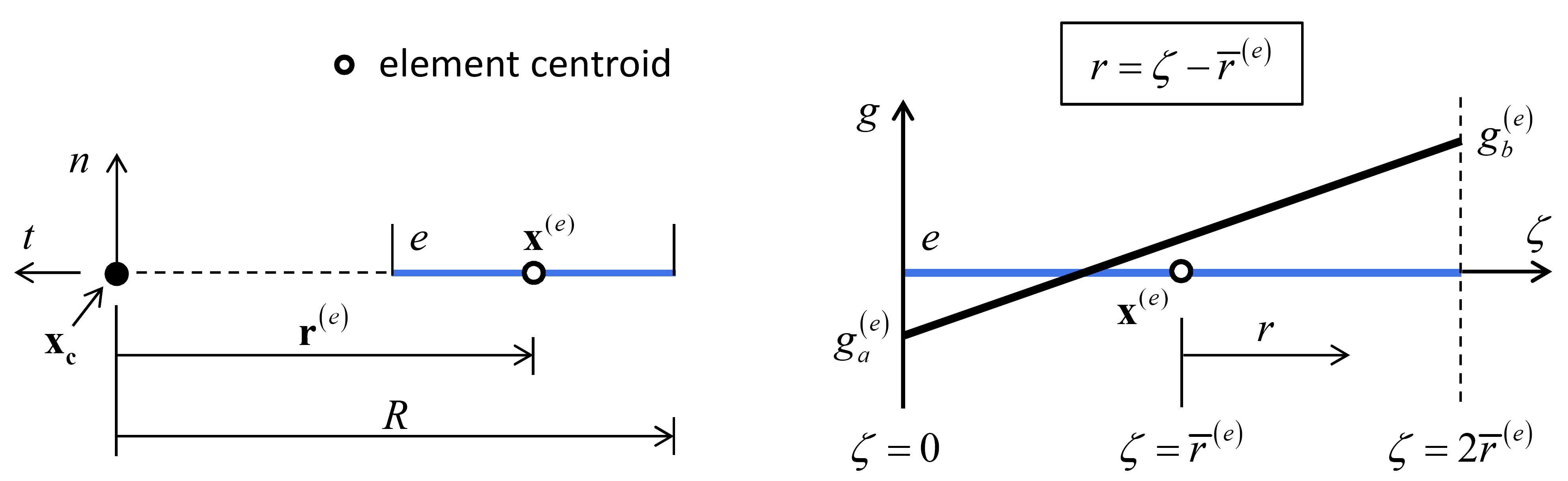
Figure 14: Variation of interface gap over a typical 2D element.
The element is mapped into one of the following three cases (in order): (1) the gap changes sign within the element (\(g_{a}^{\left(e\right)} g_{b}^{\left(e\right)} <0\)); (2) the gap remains positive or zero \(\left(g_{a}^{\left(e\right)} \ge 0{\rm \; and\; }g_{b}^{\left(e\right)} \ge 0\right)\); or (3) the gap remains negative (\(g_{a}^{\left(e\right)} \le 0\) and \(g_{b}^{\left(e\right)} \le 0\)).
The integrals in Equation (30) are expressed in the element system by
where the \(g\left(r\right)\) term of the interface normal stress of Equation (17) is expressed via Equation (31). These integrals are evaluated analytically for each case to yield (with the superscript \(\left(e\right)\) notation dropped for the \(g_{a}\), \(g_{b}\), and \(\bar{r}\) terms):
For the 3D model, it is assumed that the normal stress is constant over the element and equal to its value at the element centroid[4] such that
where \(g^{\left(e\right)}\) is the gap at the element centroid obtained by evaluating Equation (10) at the element centroid.
Usage and Verification Examples
The “Rock Testing” example application demonstrates compressive and tensile strength tests applied to simple BPMs using the linear parallel bond and flat joint contact models.
Endnotes
| [1] | A crack is a disk for the 3D model and a linear segment of unit-thickness depth for the 2D model. A crack has failure mode (tensile or shear) and geometric information (size, position, normal direction and gap). The size is two times the element radius (which is the radius giving the same area as the element), or the element length for the 2D model. The position, normal direction and gap are updated to correspond with material motion subsequent to bond breakage. Cracks are displayed by the crack-monitoring package (see section “Crack Monitoring” in [Potyondy2017]). |
| [2] | The kinematic formulation approximates the motion of two notional surfaces, each of which is connected rigidly to a piece of a body. A limitation of the current formulation is that when two bodies joined by a flat-joint contact are moved tangentially to one another, the interface gap increases (because \(g_s\) increases). It may be possible to remove this limitation by introducing an alternative interface coordinate system that does not rotate under the above condition. |
| [3] | It is assumed that the shear stress arising from relative twist rotation is constant over the element and equal to its value at the element centroid. An inaccuracy introduced by this assumption is that the twisting moment is zero with respect to the element centroid. The interface shear stress arising from relative twist rotation actually varies linearly over the element, which makes the twisting moment nonzero with respect to the element centroid. As a result, the twisting moment at the center of the interface converges to the correct value from below as the discretization is refined. A similar assumption and associated inaccuracy exists for the bending moment of the 3D flat-joint model. |
| [4] | An inaccuracy introduced by this assumption is that the bending moment is zero with respect to the element centroid. The interface normal stress actually varies linearly over the element, which makes the bending moment nonzero with respect to the element centroid. As a result, the bending moment at the center of the interface converges to the correct value from below as the discretization is refined. A similar assumption and associated inaccuracy exists for the twisting moment of the 3D flat-joint model. |
Model Summary
An alphabetical list of the flat-joint contact model methods is given here. An alphabetical list of the flat-joint contact model properties is given here.
References
| [Potyondy2017] | (1, 2, 3) Potyondy, D. O. “Material-Modeling Support in PFC [fistPkg25],” Itasca Consulting Group, Inc., Technical Memorandum ICG7766-L (March 16, 2017), Minneapolis, Minnesota. |
| [Potyondy2016] | Potyondy, D. (2016) “Flat-Joint Contact Model [version 1],” Itasca Consulting Group, Inc., Minneapolis, MN, Technical Memorandum 5-8106:16TM47, October 12, 2016. |
| [Potyondy2013] | Potyondy, D. (2013) “PFC3D Flat-Joint Contact Model (version 1),” Itasca Consulting Group, Inc., Minneapolis, MN, Technical Memorandum ICG7234-L, June 25, 2013. |
| [Potyondy2012a] | Potyondy, D. (2012a) “PFC2D Flat-Joint Contact Model,” Itasca Consulting Group, Inc., Minneapolis, MN, Technical Memorandum ICG7138-L, July 26, 2012. |
| [Potyondy2012b] | Potyondy, D.O. (2012b) “A Flat-Jointed Bonded-Particle Material for Hard Rock,” paper ARMA 12-501 in Proceedings of 46th U.S. Rock Mechanics/Geomechanics Symposium, Chicago, USA, 24–27 June 2012. |
| Was this helpful? ... | PFC © 2021, Itasca | Updated: Feb 25, 2024 |