
Linear Model
The linear model with inactive dashpots and a reference gap of zero corresponds with the model of [Cundall1979a]. It is a linear-based model that can be installed at both ball-ball and ball-facet contacts, and is referred to in commands and FISH by the name linear.
Introduction
The linear model provides linear and dashpot components that act in parallel with one another. The linear component provides linear elastic (no-tension) frictional behavior, while the dashpot component provides viscous behavior. Both components act over a vanishingly small area, and thus transmit only a force.
Behavior Summary
The linear model provides the behavior of an infinitesimal interface that does not resist relative rotation so that the contact moment equals zero \((\mathbf{M_{c}} \equiv 0)\). The contact force is resolved into linear and dashpot components \((\mathbf{F_{c}} = \mathbf{F^{l}} + \mathbf{F^{d}})\). The linear component provides linear elastic (no-tension), frictional behavior, while the dashpot component provides viscous behavior (see Figure 1). The linear force is produced by linear springs with constant normal and shear stiffnesses, \(k_n\) and \(k_s\). The dashpot force is produced by dashpots with viscosity given in terms of the normal and shear critical-damping ratios, \(\beta_n\) and \(\beta_s\). The linear springs act in parallel with the dashpots. A surface gap, \(g_s\), is defined as the difference between the contact gap \(g_c\) and the reference gap \(g_r\) so that when the reference gap is zero, the notional surfaces coincide with the piece surfaces (see Figure 2). The contact is active if and only if the surface gap is less than or equal to zero; the force-displacement law is skipped for inactive contacts.
The linear springs cannot sustain tension, and slip is accommodated by imposing a Coulomb limit on the shear force using the friction coefficient, \(\mu\). Denote the normal and shear components of the linear force by \(F_{n}^{l}\) and \(\mathbf{F_{s}^{l}}\), respectively. \(F_{n}^{l}\) is updated either in an absolute sense based on the surface gap, or incrementally based on the surface-gap increments, with the update type controlled by the normal-force update mode, \(M_{l}\). \(\mathbf{F_{s}^{l}}\) is always updated incrementally based on relative shear-displacement increments.
The dashpot force is affected by the dashpot mode, \(M_{d}\), which provides four combinations of normal and shear behavior. Denote the normal and shear components of the dashpot force by \(F_{n}^{d}\) and \(F_{s}^{d}\), respectively. The normal-behavior mode can be either full or no-tension, where full means that the entire dashpot load is assigned and no-tension means that \(F_{n}^{d}\) is capped to insure that the total normal force (\(F_{n}^{l} + F_{n}^{d}\)) does not become tensile. The shear-behavior mode can be either full or slip-cut, where slip-cut means that \(F_{s}^{d}\) is set to zero if the linear spring is sliding.
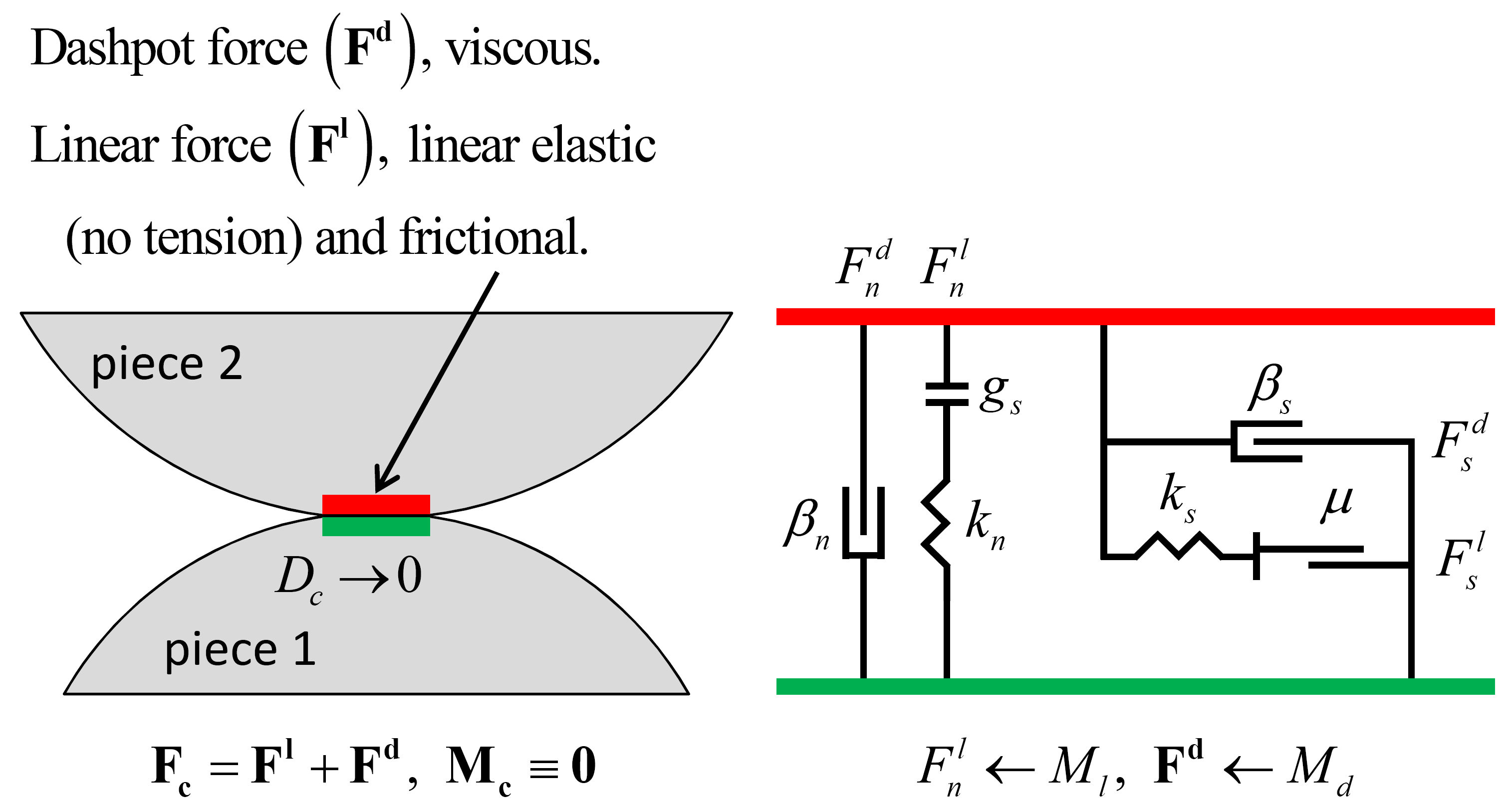
Figure 1: Behavior and rheological components of the linear model.
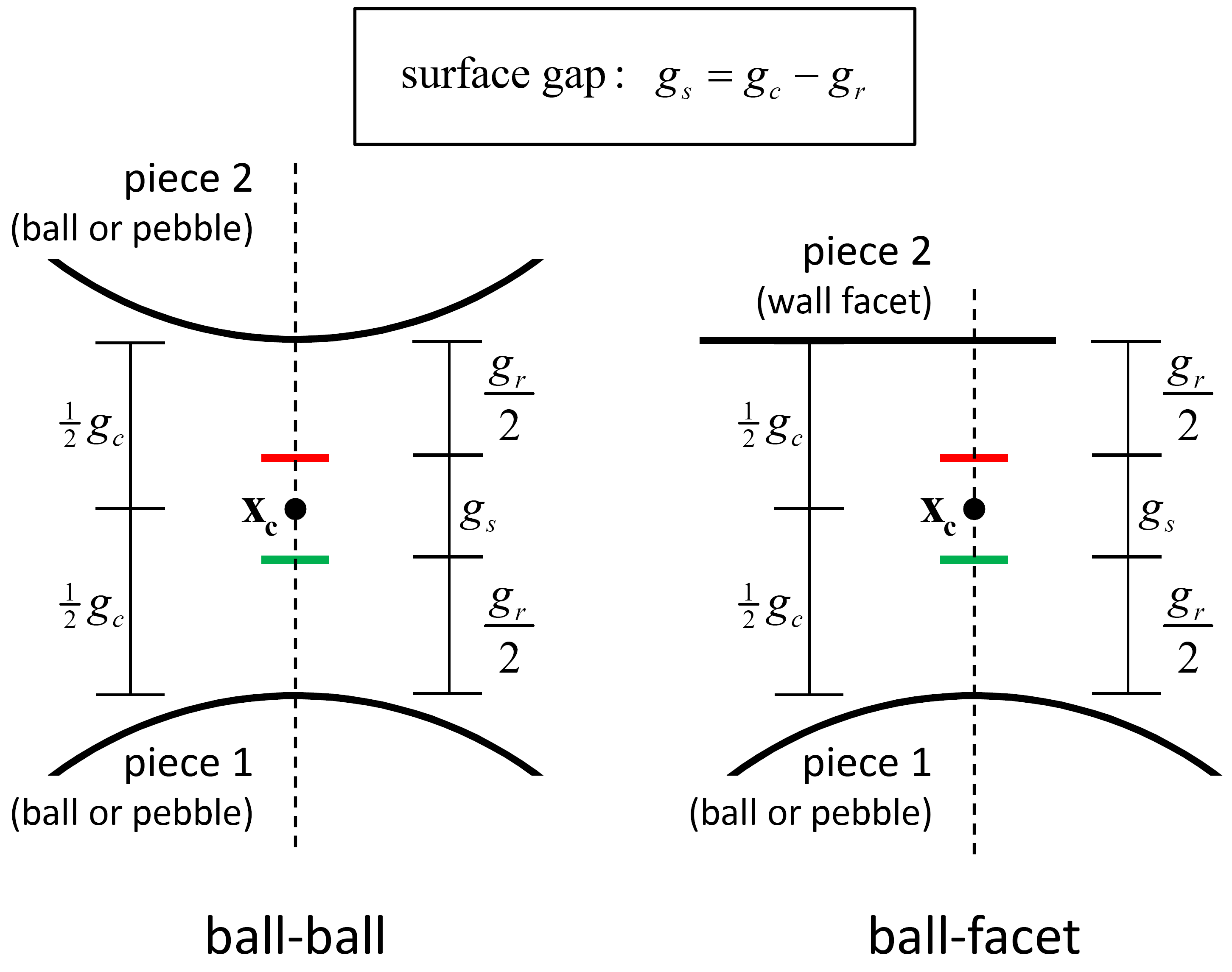
Figure 2: Surface gap for the linear-based models.
Activity-Deletion Criteria
A contact with the linear model is active if and only if the surface gap is less than or equal to zero. The force-displacement law is skipped for inactive contacts. The surface gap is shown in Figure 2. When the reference gap is zero, the notional surfaces coincide with the piece surfaces.
Force-Displacement Law
The relative displacement increment at the contact during a timestep \(\Delta t\) is given by \(\Delta \delta _{n}\) and \(\Delta \pmb{δ}_{\mathbf{s}}\) in this equation of the “Contact Resolution” section. If the contact transitions from inactive to active during the current timestep, then only the portion of this increment that occurs while the surface gap is negative is used to perform the incremental update of the normal and shear forces The relative displacement increment is adjusted:
where \((g_s)_{o}\) is the surface gap at the beginning of the timestep. The adjusted increment is used in the force-displacement law.
The force-displacement law for the linear model updates the contact force and moment:
where \(\mathbf{F^{l}}\) is the linear force and \(\mathbf{F^{d}}\) is the dashpot force. Both forces are resolved into normal and shear forces:
where \(F_{n}^{\left\{l,d\right\}} >0\) is tension. Both shear forces lie on the contact plane, and the linear shear force is expressed in the contact plane coordinate system:
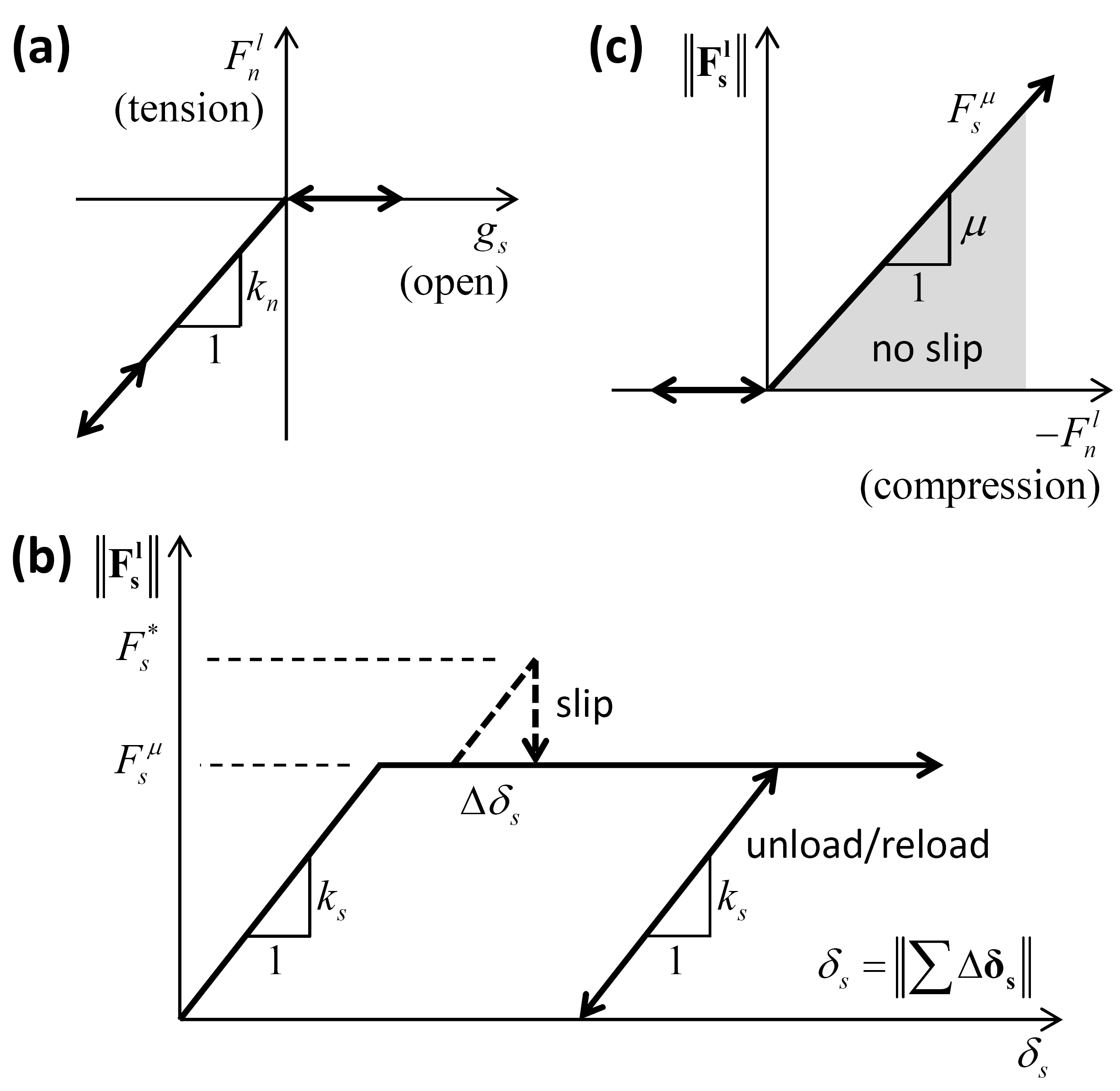
Figure 3: Force-displacement law for the linear component of the unbonded linear-based models: (a) normal force versus surface gap, (b) shear force versus relative shear displacement, and (c) slip envelope.
The force-displacement law for the linear model consists of the following steps (see Figure 3).
Update the linear normal force based on the normal-force update mode:
(5)\[\begin{split}F_{n}^{l} = \left\{ \begin{array}{rl} \left\{ \begin{array}{rl} k_n g_s, & g_s < 0 \\ 0, & \mbox{otherwise} \end{array} \right. , & \mbox{$M_l = 0$ (absolute update)} \\ \min\left( (F_n^l)_o + k_n\Delta\delta_n, 0 \right), & \mbox{$M_l = 1$ (incremental update)} \end{array} \right.\end{split}\]where \(\left(F_{n}^{l} \right)_{o}\) is the linear normal force at the beginning of the timestep. For both update modes, no-tension behavior is enforced so that the linear normal force is always compressive, and it is nonzero only when the surface gap is negative (as shown in Figure 3(a)).
Update the linear shear force as follows. Compute a trial shear force (see Figure 4):
(6)\[\mathbf{F_{s}^{*}} = \left( \mathbf{F_{s}^{l}} \right)_{o} - k_{s} \Delta \pmb{δ} _\mathbf{s}\]where \(\left( \mathbf{F_{s}^{l}} \right)_{o}\) is the linear shear force at the beginning of the timestep, and \(\Delta \pmb{δ} _\mathbf{s}\) is the adjusted relative shear-displacement increment of Equation (1). Compute the shear strength:
(7)\[F_{s}^{\mu } =-\mu F_{n}^{l} .\]Update the linear shear force:
(8)\[\begin{split}\mathbf{F_s^l} = \left\{ \begin{array}{rl} \mathbf{F_s^*} , & \| \mathbf{F_s^*} \| \le F_s^{\mu} \\ F_s^{\mu} \bigl( \mathbf{F_s^*} / \| \mathbf{F_s^*} \| \bigr), & \mbox{otherwise.} \end{array} \right.\end{split}\]Update the slip state:
(9)\[\begin{split}s = \left\{ \begin{array}{rl} \mbox{true}, & \| \mathbf{F_s^l} \| = F_s^{\mu} \\ \mbox{false}, & \mbox{otherwise.} \end{array} \right.\end{split}\]If the slip state is true, then the contact is sliding. Whenever the slip states changes, the slip_change callback event occurs.
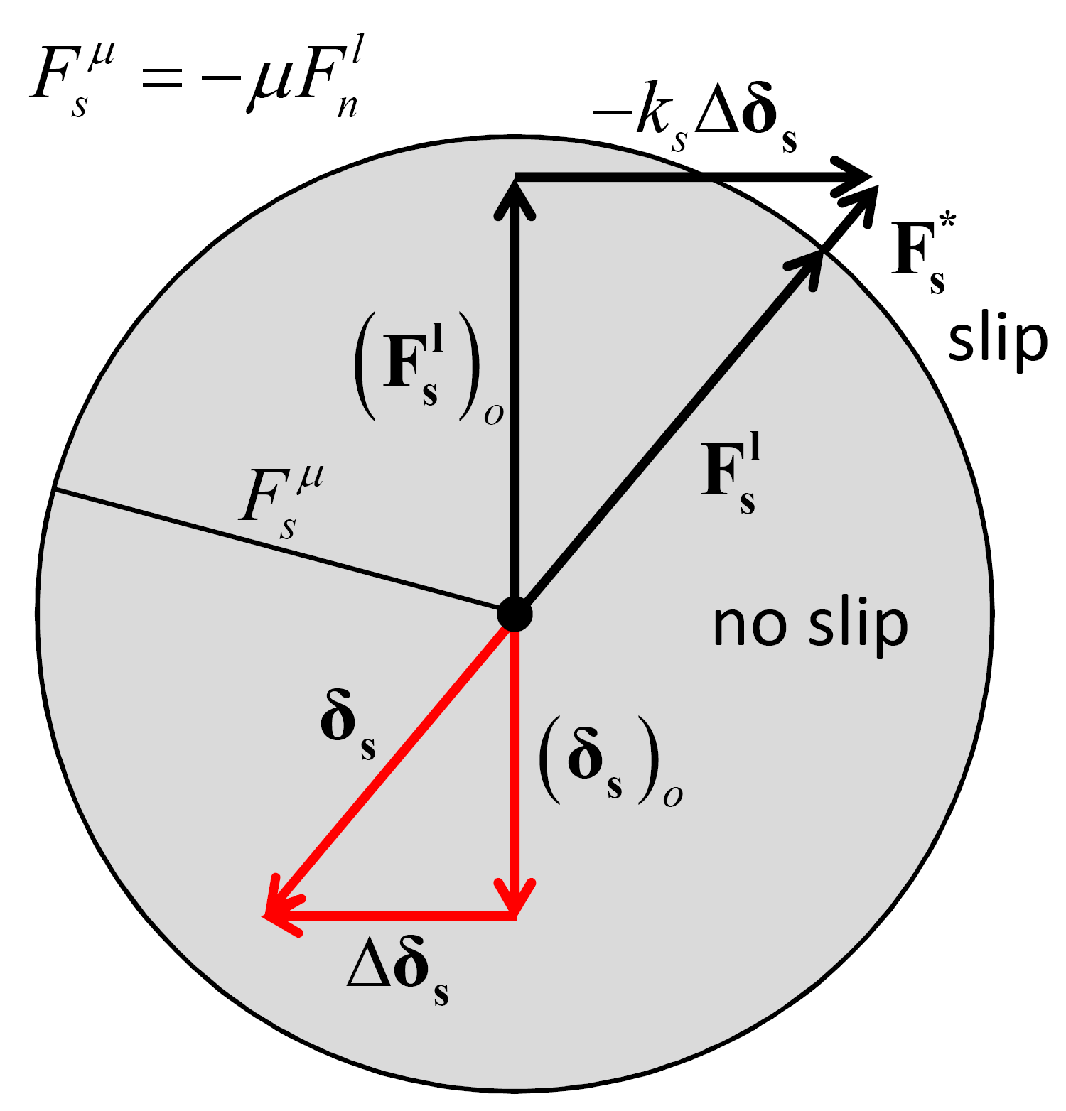
Figure 4: Update of the linear shear force and relative shear displacement during slip of linear-based models.
Update the dashpot normal force based on the dashpot behavior mode:
(10)\[\begin{split}\begin{array}{l} F_n^d = \left\{ \begin{array}{rl} F^*, & \mbox{$M_d = \{ 0, 2 \}$ (full normal)} \\ \min\left( F^*, -F_n^l \right), & \mbox{$M_d = \{ 1, 3 \}$ (no-tension normal)} \end{array} \right. \\[3mm] \mbox{with }\quad F^* = \left( 2 \beta_n \sqrt{m_c k_n} \right) \dot{\delta}_n \\ \hskip{15mm} m_c = \left\{ \begin{array}{rl} \displaystyle\frac{m^{(1)} m^{(2)}} {m^{(1)} + m^{(2)}}, & \mbox{ball-ball} \\ m^{(1)}, & \mbox{ball-facet} \end{array} \right. \end{array}\end{split}\]where \(m^{(b)}\) is the mass of body \((b)\) and \(\dot{\delta}_n\) is the relative normal translational velocity of this equation of the “Contact Resolution” section. In this expression, \(F^*\) is the entire dashpot load. For the dashpot normal-behavior mode of no-tension, \(F_n^d\) is capped to ensure that the total normal force \((F_n^l + F_n^d)\) does not become tensile.
Update the dashpot shear force based on the dashpot behavior mode:
(11)\[\begin{split}\begin{array}{l} \mathbf{F_s^d} = \left\{ \begin{array}{rl} \left( 2 \beta_s \sqrt{m_c k_s} \right) \dot{\pmb{δ}}_\mathbf{s}, & \mbox{$s =$ false or $M_d = \{ 0, 1 \}$ (full shear)} \\ \mathbf{0}, & \mbox{$s =$ true and $M_d = \{ 2, 3 \}$ (slip-cut)} \end{array} \right. \\[3mm] \mbox{with }\quad m_c = \left\{ \begin{array}{rl} \displaystyle\frac{m^{(1)} m^{(2)}} {m^{(1)} + m^{(2)}}, & \mbox{ball-ball} \\ m^{(1)}, & \mbox{ball-facet} \end{array} \right. \end{array}\end{split}\]where \(m^{(b)}\) is the mass of body \((b)\) and \(\dot{\pmb{δ}}_\mathbf{s}\) is the relative shear translational velocity of this equation of the “Contact Resolution” section. For the dashpot shear-behavior mode of slip-cut, \(\mathbf{F_s^d}\) is set to zero if the linear spring is sliding \(\mbox{($s =$ true)}\).
Energy Partitions
The linear model provides three energy partitions:
- strain energy, \(E_{k}\), stored in the linear springs;
- slip energy, \(E_{\mu}\), defined as the total energy dissipated by frictional slip; and
- dashpot energy, \(E_{\beta}\), defined as the total energy dissipated by the dashpots.
If energy tracking is activated, these energy partitions are updated as follows:
Update the strain energy:
(12)\[{\rm E} _{k} =\frac{1}{2} \left(\frac{\left(F_{n}^{l} \right)^{2} }{k_{n} } +\frac{\left\| \mathbf{F_{s}^{l}} \right\| ^{2} }{k_{s} } \right).\]Update the slip energy:
(13)\[\begin{split}\begin{array}{l} {E_{\mu } :=E_{\mu } - {\tfrac{1}{2}} \left(\left(\mathbf{F_{s}^{l}} \right)_{o} +\mathbf{F_{s}^{l}} \right)\cdot \Delta \pmb{δ} _\mathbf{s}^{\mu } } \\ {{\rm with}\qquad \Delta \pmb{δ} _\mathbf{s}^{\mu } =\Delta \pmb{δ} _\mathbf{s} -\Delta \pmb{δ} _\mathbf{s}^{k} =\Delta \pmb{δ} _\mathbf{s} -\left(\frac{\mathbf{F_{s}^{l}} -\left(\mathbf{F_{s}^{l}} \right)_{o} }{k_{s} } \right)} \end{array}\end{split}\]where \(\left(\mathbf{F_{s}^{l}} \right)_{o}\) is the linear shear force at the beginning of the timestep, and the adjusted relative shear-displacement increment of Equation (1) has been decomposed into an elastic \(\left(\Delta \pmb{δ} _\mathbf{s}^{k} \right)\) and a slip \(\left(\Delta \pmb{δ} _\mathbf{s}^{\mu } \right)\) component. The dot product of the slip component and the average linear shear force occurring during the timestep gives the increment of slip energy.
Update the dashpot energy:
(14)\[E_{\beta } :=E_{\beta } - \mathbf{F^{d}} \cdot \left(\dot{\pmb{δ} }{\kern 1pt} {\kern 1pt} \Delta t\right)\]where \(\dot{\pmb{δ} }\) is the relative translational velocity of this equation of the “Contact Resolution” section.
Additional information, including the keywords by which these partitions are referred to in commands and FISH, is provided in the table below.
| Keyword | Symbol | Description | Range | Accumulated |
|---|---|---|---|---|
| Linear Group: | ||||
energy‑strain |
\(E_{k}\) | Strain energy | \([0.0,+\infty)\) | NO |
energy‑slip |
\(E_{\mu}\) | Total energy dissipated by slip | \((-\infty,0.0]\) | YES |
| Dashpot Group: | ||||
energy‑dashpot |
\(E_{\beta}\) | Total energy dissipated by dashpots | \((-\infty,0.0]\) | YES |
Properties
The properties defined by the linear contact model are listed in the table below as a concise reference; see the Contact Properties section for a description of the information in the table columns. The mapping from the surface inheritable properties to the contact model properties is also discussed below.
| Keyword | Symbol | Description | Type | Range | Default | Modifiable | Inheritable |
|---|---|---|---|---|---|---|---|
| linear | Model name | ||||||
| Linear Group: | |||||||
| kn | \(k_n\) | Normal stiffness [force/length] | FLT | \([0.0,+\infty)\) | 0.0 | YES | YES |
| ks | \(k_s\) | Shear stiffness [force/length] | FLT | \([0.0,+\infty)\) | 0.0 | YES | YES |
| fric | \(\mu\) | Friction coefficient [-] | FLT | \([0.0,+\infty)\) | 0.0 | YES | YES |
| rgap | \(g_r\) | Reference gap [length] | FLT | \(\mathbb{R}\) | 0.0 | YES | NO |
| lin_mode | \(M_l\) | Normal-force update mode [-] | INT | \(\{0,1\}\) | 0 | YES | NO |
| \(\;\;\;\;\;\;\begin{cases} \mbox{0: update is absolute} \\ \mbox{1: update is incremental} \end{cases}\) | |||||||
| emod | \(E^*\) | Effective modulus [force/area] | FLT | \([0.0,+\infty)\) | 0.0 | NO | N/A |
| kratio | \(\kappa^*\) | Normal-to-shear stiffness ratio [-] | FLT | \([0.0,+\infty)^*\) | 0.0\(^*\) | NO | N/A |
| \(\kappa^* \equiv \frac{k_n}{k_s}\) | |||||||
| lin_slip | \(s\) | Slip state [-] | BOOL | {false,true} | false | NO | N/A |
| \(\;\;\;\;\;\;\begin{cases} \mbox{true: slipping} \\ \mbox{false: not slipping} \end{cases}\) | |||||||
| lin_force | \(\mathbf{F^l}\) | Linear force (contact plane coord. system) | VEC | \(\mathbb{R}^3\) | \(\mathbf{0}\) | YES | NO |
| \(\left( -F_n^l,F_{ss}^l,F_{st}^l \right) \quad \left(\mbox{2D model: } F_{ss}^l \equiv 0 \right)\) | |||||||
| user_area | \(A\) | Constant area [length*length] | FLT | \((0.0,+\infty)\) | 0.0 | YES | NO |
| Dashpot Group: | |||||||
| dp_nratio | \(\beta_n\) | Normal critical damping ratio [-] | FLT | \([0.0,1.0]\) | 0.0 | YES | NO |
| dp_sratio | \(\beta_s\) | Shear critical damping ratio [-] | FLT | \([0.0,1.0]\) | 0.0 | YES | NO |
| dp_mode | \(M_d\) | Dashpot mode [-] | INT | {0,1,2,3} | 0 | YES | NO |
| \(\;\;\;\;\;\;\begin{cases} \mbox{0: full normal & full shear} \\ \mbox{1: no-tension normal & full shear} \\ \mbox{2: full normal & slip-cut shear} \\ \mbox{3: no-tension normal & slip-cut shear} \end{cases}\) | |||||||
| dp_force | \(\mathbf{F^d}\) | Dashpot force (contact plane coord. system) | VEC | \(\mathbb{R}^3\) | \(\mathbf{0}\) | NO | NO |
| \(\left( -F_n^d,F_{ss}^d,F_{st}^d \right) \quad \left(\mbox{2D model: } F_{ss}^d \equiv 0 \right)\) | |||||||
| \(^*\) By convention, \(\kappa^* = 0.0\) if either the normal or the shear stiffness is 0. | |||||||
Note
Out-of-balance forces acting on bodies are accumulated during force-displacement calculations. Modifying the forces stored in the contact models will not alter them instantaneously. Therefore, any change to \(\mathbf{F^l}\) may only be effective during the next force-displacement calculation. When \(M_l = 0\), the normal component of the linear force is automatically overridden during the next force-displacement calculation.
Surface Property Inheritance
The linear stiffnesses, \(k_n\) and \(k_s\), and the friction coefficient, \(\mu\), may be inherited from the contacting pieces. Remember that for a property to be inherited, the inheritance flag for this property must be set to true (default), and both contacting pieces must hold a property with the exact same name.
The linear stiffnesses are inherited, assuming that both pieces’ stiffness act in series (Figure 5):
where \((1)\) and \((2)\) denote the properties of piece 1 and 2, respectively.
The friction coefficient is inherited using the minimum of the values set for the pieces:
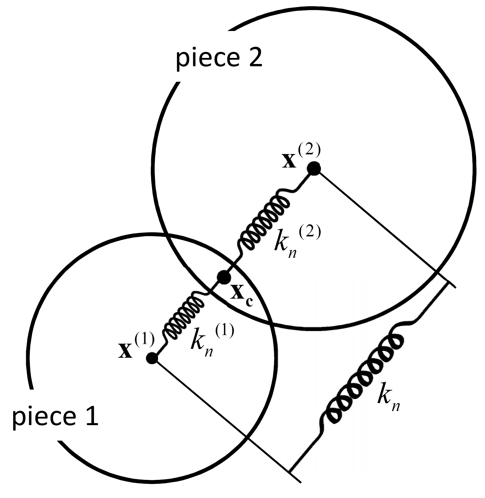
Figure 5: Relation of normal stiffness to piece normal stiffnesses for the linear model. The normal stiffness corresponds with the piece normal stiffnesses acting in series.
Methods
| Method | Arguments | Symbol | Type | Range | Default | Description |
|---|---|---|---|---|---|---|
| area | Set user_area to the area | |||||
| deformability | Set deformability | |||||
| emod | \(E^*\) | FLT | \([0.0,+\infty)\) | N/A | Effective modulus | |
| kratio | \(\kappa^*\) | FLT | \([0.0,+\infty)^*\) | N/A | Normal-to-shear stiffness ratio | |
| \(^*\) By convention, setting \(\kappa^* = 0.0\) sets \(k_s = 0.0\) but does not alter \(k_n\). | ||||||
Area
Set the user_area property via the current contact area. This operation means that the contact area stays constant and is fixed independent of changes to the piece sizes/geometries. In order for the stiffnesses to be recomputed accounting for this area, one should subsequently call the deformabilty method.
Deformability
The deformability of a homogeneous, isotropic, and well-connected granular assembly experiencing small-strain deformation can be fit by an isotropic material model, which is described by the elastic constants of Young’s modulus \((E)\) and Poisson’s ratio \((\nu)\). \(E\) and \(\nu\) are emergent properties that can be related to the effective modulus \((E^{*})\) and the normal-to-shear stiffness ratio \((\kappa^* \equiv k_n/k_s)\) at the contact as follows: \(E\) is related to \(E^{*}\), with \(E\) increasing as \(E^{*}\) increases; \(\nu\) is related to \(\kappa^{*}\), with \(\nu\) increasing up to a limiting positive value as \(\kappa^{*}\) increases. These relationships are obtained by specifying \(E^{*}\) and \(\kappa^{*}\) as the arguments of the deformabilty method, which sets:
The first term in this expression is obtained by equating the normal stiffness to the axial stiffness of the volume of material shown in Figure 6. Note that the user_area property can be used to override this volume, specifying the area of the contact directly.
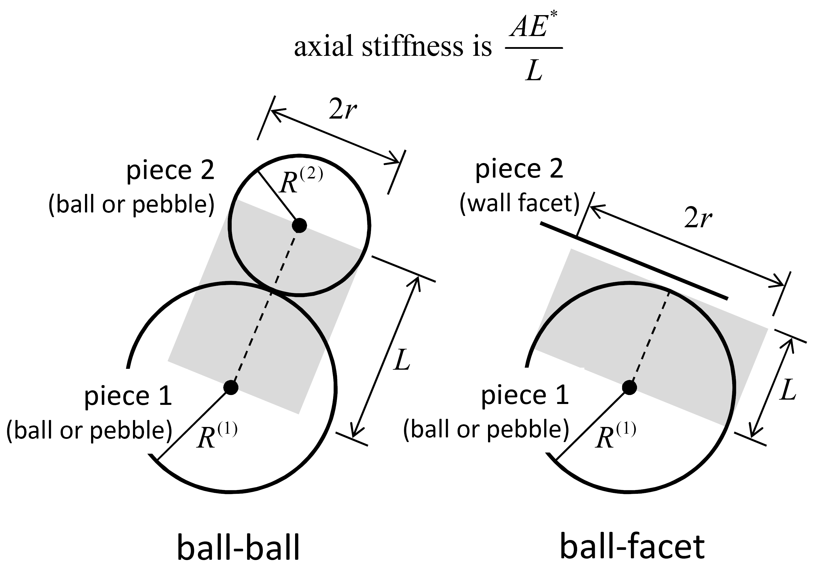
Figure 6: Volume of material associated with contact.
Callback Events
| Event | Array Slot | Value Type | Range | Description |
|---|---|---|---|---|
| contact_activated | Contact has become active | |||
| 1 | C_PNT | N/A | Contact pointer | |
| slip_change | Slip state has changed | |||
| 1 | C_PNT | N/A | Contact pointer | |
| 2 | INT | {0,1} | Slip change mode | |
| \(\;\;\;\;\;\;\begin{cases} \mbox{0: slip has initiated} \\ \mbox{1: slip has ended} \end{cases}\) | ||||
Usage and Verification Examples
The tutorials “Balls in a Box” and “Clumps in a Box” demonstrate the use of the linear model.
Calibration of the dashpot parameters to achieve a target impact coefficient of restitution is demonstrated in “Linear Contact Model: Calibrating the Normal Critical Damping Ratio.”
to do items below
Model Summary
An alphabetical list of the linear model methods is given here. An alphabetical list of the linear model properties is given here.
References
| [Cundall1979a] | Cundall P.A., and O.D.L. Strack. “A Discrete Numerical Model for Granular Assemblies,” Géotechnique, 29, 47-65, 1979. |
| Was this helpful? ... | PFC © 2021, Itasca | Updated: Feb 25, 2024 |