
Commands, a Rationale
At this juncture, users who have reviewed the preceding material should have a good working understanding of program commands and how to use the Console pane to issue them. However, it may not be entirely clear why the program is designed to utilize commands this way in the first place. The following discussions are provided to give insight into this question.
Why A Command-Driven Interface?
Whether generated interactively or manually, the basic description of any FLAC3D model is a data file. A data file is a standard text file containing commands that completely specify a FLAC3D model, from model creation to additional sequential operations required to undertake physical simulations.
At first exposure, the fact that FLAC3D uses data files to describe the model may seem antiquated, perhaps a relic of 1970s program design. To the contrary, this form of model description has proven to be quite valuable and is considered an integral part of what makes FLAC3D, and Itasca codes in general, powerful modeling tools. As our user interface design matures, our goal is not to remove the command-driven interface but, instead, to simplify its use, making simulations easier to undertake while retaining the flexibility this design embodies.
Below are a few reasons that using a data file description is advantageous.
Compact representation
Even the most complex models can be created by a set of data files that are generally not more than a few hundred lines in length. In fact, the vast majority of models are far smaller. This fact means that the complete description of your FLAC3D model resides in a text file that is only a few kilobytes in size. As a result, it is trivial to share your model with others, email it to Itasca for support, archive your model for future reference, and use versioning software to track changes.
Repeatability
Itasca works very hard to ensure that the same version of the code and the same data file will always produce the same result to machine precision. This means that when you send Itasca, your colleagues, or your clients a data file, you know that the result will be unchanging. Thus it is not necessary to archive the complete results of a modeling effort, which may be many gigabytes of save and result files. Instead, one can just retain the data file and the code version used to execute it.
History and Path Dependence
Except for the most trivial models using the simplest of materials, the path used to reach the solution is a very important part of the model description. A data file allows the sequence of events to be described clearly and flexibly. Many programs may offer excavation sequence options, but the data file allows any sequence of events to be made if necessary. This includes changes to boundary conditions, changes to material properties, changes to fluid interactions, etc. as well as changes to the excavation sequencing. If one were to design a graphical user interface to include the entire list of options available via a data file, the result would be complex, requiring clumsy tools to edit and change.
Flexibility
The data file allows the user maximum flexibility in how they choose to create and process a model, including the order in which things are specified. While there is a standard sequence of simulation steps recommended for simple models (e.g., geometry creation, naming of regions, material and property specification, boundary conditions, initial conditions, solving, excavating, solving, etc.), every model is different. Often complex models require modifications to the standard simulation progression. Itasca is committed to the idea of not constraining users to a small set of simulation options, providing users with the ability and tools to undertake physical simulations in the way they see fit.
Scripting
The ability to combine model-creation commands with scripting in FLAC3D is tremendously powerful. For instance, an entire class of models can be investigated by trivially changing a set of initial parameters within a data file. Application of complex sequences, geometries, property distributions, etc. may be automated with a script in a way that would be very time consuming and difficult to replicate in a traditional graphical user interface. In addition, in-depth model querying and the inclusion of new physical phenomena, not included in FLAC3D, can be introduced via user-created scripts that execute during cycling.
The downside to such a command-driven interface is that it can be imposing for new users, who may have the impression that mastery of a large number of complex commands is necessary to undertake the simplest of modeling efforts. In truth, the learning curve is faster than being confronted by a complex graphical user interface that has numerous tools with a plethora of buttons in different panes—something we have all experienced. The commands have been purposefully structured using descriptive and consistent terminology, making it easy to read a data file and understand the operations it invokes. In addition, interactive command documentation is available as you create and edit a data file from within FLAC3D, simplifying the process substantially.
In order to make creating and editing data files as easy as possible, FLAC3D contains the following features:
Why FISH?
Introduction
FISH is a built-in scripting language that gives the FLAC3D user powerful control over most every aspect of program operation. FISH is short for “FLAC-ISH” (or the language of FLAC), the code for which it was first developed. Now, in addition to FLAC and FLAC3D, FISH is also integrated into all Itasca commercial programs.
FISH is embedded deeply into FLAC3D at nearly every level. It can be used to parameterize data files so that a number of varying cases can be built into the same basic model. Every data type that makes up a FLAC3D model is also available for FISH to manipulate directly—before, after, and during the solution. This means that not only can FISH be used to create custom complex models and customized results, it can also be used to add custom physics to the solution process that is not part of the standard package.
FISH includes constructs to embed FLAC3D commands within FISH functions (see the command – end command block in the example shown in the Run Control section). parenthetical here awkward, unsure of how to edit?
FISH is a semi-compiled language that uses dynamic typing for variables – syntax and use is similar to (but not exactly the same as) Python. It has been created to be very simple for small needs, but it provides structure and data types needed to support large and complex programs if necessary.
The following illustrations give just an idea of the power of FISH. More complete information is available in the sections Tutorial: Working with FISH and FISH Scripting Reference. Examples below are given to represent five general areas of application:
Model Creation: Property Initialization
The following FISH routine specifies a bulk modulus as a function of current mechanical pressure in the zones.
fish define iniBulk(a,b)
    loop foreach zone zone.list
        local stress = zone.stress.effective(zone)
        local pressure = tensor.trace(stress)/3
        local bulk = a + b*math.sqrt(pressure)
        zone.prop(zone,'bulk') = bulk
    end_loop
end
[iniBulk(1e7,1e6)]
This is a particularly simple example for the purposes of illustration.
Parameterization: Varying Model Geometry
For this example, we create a simple model of a tunnel interactively using the 2D extrusion tool. The tool’s data and the resulting zones are shown below. Note that the points used for tunnel are marked in green as a group named Tunnel.
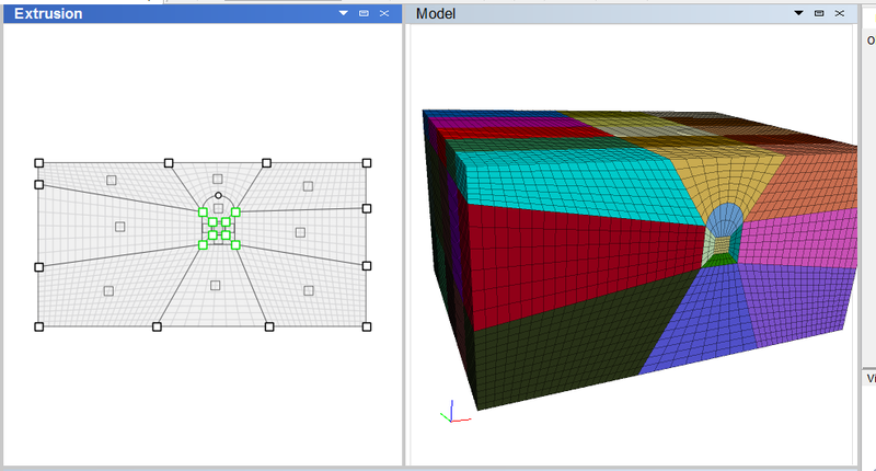
Using this as a template, we use the State Record pane to create a data file named create_tunnel.dat that reproduces this geometry. Then we can create a parameterized data file that allows us to test various tunnel locations while only changing one value (tunnel_height defined on line 3).
model new
; Specify model parameters
[tunnel_height = 20.0]
program call 'create_tunnel' ; Load template of model geometry
; The template created has the tunnel base at 25,
; and tunnel points are marked with group 'Tunnel'
; Move points
extrude point transform translate 0 [tunnel_height-25.0] range group 'Tunnel'
; Generate zones
zone generate from-extruder
As seen on line 8, this example demonstrates the ability to substitute FISH values and expressions anywhere a value is expected within a data file.
Note that things like material properties, tunnel cross-section, and almost anything involved in the model can be parameterized in such a fashion—sometimes simply with parameter replacement in the data file as seen here, sometimes with the use of FISH functions (as seen above in the Model Creation section). This allows quick and easy exploration of the parameter space of a model that requires set up once and only once.
Custom Visualization: Positing a Plane of Weakness
Perhaps the most common use of FISH is to customize model results. Providing this ability was the original motivation for its introduction into Itasca software. FISH allows the user to plot any quantity of interest in the model without requiring the addition of a bewildering variety of rarely used options on a menu tree somewhere. The following is an example of a script that calculates, over the entire model, the normal and shear stress components on a particular plane orientation. It also creates a flag (fail, line 9) that indicates if failure would occur on that plane, given a specific friction angle (tauCrit, line 8).
fish automatic-create off
fish define shearNormal(dip,dd,fric)
    local norm = math.normal.from.dip.ddir(dip*math.degrad,dd*math.degrad)
    loop foreach local zone zone.list
        local stress = zone.stress(zone)
        local traction = stress*norm
        local normalStress = math.dot(traction,norm)
        local shear = math.mag(traction - (norm*normalStress))
        local tauCrit = -normalStress*math.tan(fric*math.degrad)
        local fail = shear > tauCrit

        zone.extra(zone,1) = fail
        zone.extra(zone,2) = normalStress
        zone.extra(zone,3) = shear
    endloop
end
[shearNormal(45,90,20)]
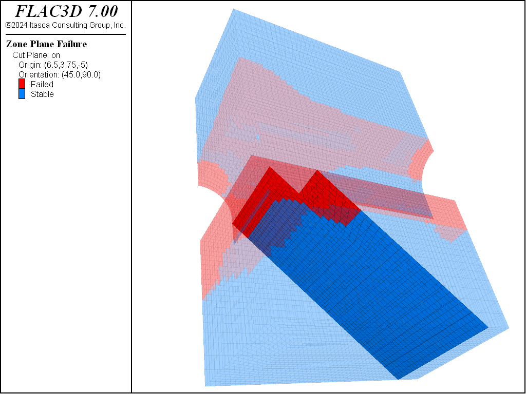
Compressive stresses are negative in FLAC3D (note the definition of tauCrit on line 8). The following is a plot of the result, looking at a cut-away plane at the same orientation, from the Pillar Loads At Intersecting Tunnels example problem. Note that FLAC3D legend entries can be customized to make the content of the plot clearer—in this case fail evaluates to Boolean values (true, false), but on the plot legend these are re-labeled Failed and Stable.
Physics Extension: Ground Freezing
FISH functions can be called during cycling/solving to solution. FISH can be invoked at any point during each calculation cycle to override or to add additional physics to the model. Each cycle is one iteration of the steps in the explicit solution scheme; placement of FISH within that sequence can be specified by command.
The following is a simple illustration of a FISH operator, groundFreezing, that could be used to model ground freezing during a coupled thermo-mechanical analysis. An operator is a special class of FISH function that can (under restrictions enforced when it is parsed) be executed using all threads available to your system.
program call 'freezezone'
fish operator groundFreezing(zone)
    ; Skip zones that are already frozen
    if zone.group(zone,'state') == 'frozen' then exit
    if zone.temp(zone) > 0.0 then exit
    freezeZone(zone)
end
This calls a FISH operator freezeZone (definition below) that actually changes the stress and stiffness of the zone and marks it as frozen.
fish operator freezeZone(zone)
    local porosity = zone.fluid.prop(zone,'porosity')
    ; Note: Assuming fully saturated
    local expansion = porosity * 0.09 * 1.0
    ;  Porosity * water expansion * saturation
    local bulk = zone.prop(zone,'bulk')
    local stress_inc = bulk * expansion
    ; Amount to increment stress
    local bulk_inc = (8.96/2.16) * porosity
    ; Ratio of ice/water bulk * porosity
    zone.prop(zone,'bulk') += bulk_inc
    ; Compressive negative!
    zone.stress(zone) -= tensor(stress_inc,stress_inc,stress_inc)
    zone.group(zone,'state') = 'frozen'
end
Freezing could be added to the solution processing with a command like the following.
fish callback add groundFreezing([::zone.list]) -100 interval 10
The groundFreezing operator is passed the list of zones to act upon.
The :: prefix indicates that the list of zones should be split into a separate call on each zone in the list using all threads.
The interval keyword is used to indicate the operator should only be exected once every 10 steps
(to further limit the effect on solution time).
The same thing can be done as part of the model solve command, as in the example below.
A command such as the following would solve to 1 year of thermal time with a ground freezing check
every 10 cycles.
model solve time-total [360*24*60*60] ...      ; 1 year (360 days) of heating.
      mechanical ratio 1e-3 ...    ; Relax solve requirements a bit for speed.
      fish-call -100 groundFreezing([::zone.list]) interval 10
                                               ; program call ground freezing.
The distinction between the two formulations shown above is that the former is global and will
take effect with any subsequent model solve command; the latter specifies execution of
FISH only for that particular issuance of model solve.
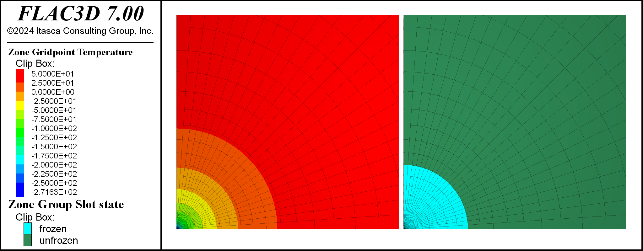
The following image displays the results when run on a modified version of the Infinite Line Heat Source in an Infinite Medium example problem.
model new
model large-strain off
model configure thermal fluid
; --- model geometry
zone create cylinder point 1 (500,0,0) ...
                     point 2 (0,1,0)  ...
                     point 3 (0,0,500) ...
                     size (48,1,24) rat 1.1 1 1
zone face skin slot 'uniform' ; Label model boundaries
zone group 'unfrozen' slot 'state' ; Initialize state marker
; --- mechanical model
zone cmodel assign elastic
zone property bulk 5e10 shear 3e10 density 2e3
zone gridpoint fix velocity-x 0 range group 'West' ; Boundary Conditions
zone gridpoint fix velocity-y 0 range group 'North' or 'South'
zone gridpoint fix velocity-z 0 range group 'Bottom'
; --- thermal model
zone thermal cmodel isotropic
zone thermal property conductivity 4 expansion 5e-6 specific-heat 1e3
zone gridpoint initialize temperature 50
zone gridpoint fix source -200 range pos-x 0 pos-z 0 ; Apply thermal sink
; --- fluid model
zone fluid cmodel assign isotropic
zone fluid property porosity 0.3
; --- settings
zone fluid active off ; No fluid coupling for this example
zone thermal implicit on
model thermal timestep fix 6.48e3
model save 'line-year0'
; --- Add ground freezing
program call 'groundfreezing'
; --- Coupled analysis
model mechanical slave on
; excerpt-solve-start
model solve time-total [360*24*60*60] ...      ; 1 year (360 days) of heating.
      mechanical ratio 1e-3 ...    ; Relax solve requirements a bit for speed.
      fish-call -100 groundFreezing([::zone.list]) interval 10
                                               ; program call ground freezing.
; excerpt-solve-end
model save 'line-year1'

program return

fish callback add groundFreezing([::zone.list]) -100 interval 10
This example is very simple but still potentially useful. More accuracy can be added, depending on the needs of the model. For example, more properties can be modified, the constitutive model can be changed to one that supports creep, and the heat of fusion required to change water to ice can be taken into account.
Run Control: Yield at Multiple Joint Angles
The following is a simplification of Uniaxial Compressive Strength of a Jointed Material Sample. Eighteen model runs are made under FISH control to create a plot of failure stress versus joint angle (which is increased by five degrees with each run, starting from 0). The entire data file required is shown below:
model new
model large-strain off
zone ratio convergence  ; use more conservative convergence criteria
program call 'cylinder' ; Load extruder description of model geometry
program call 'measure'  ; Defines 'measureStress', which measures
                        ; surface stress and stores in table
fish define triaxSolver
    loop local beta (0,90,5)
        command
            zone delete                      ; Destroy all zones
            zone generate from-extruder      ; Create new zones
            zone cmodel ubiquitous-joint     ; Assign constitutive model
            zone property bulk 1e8 shear 7e7 cohesion 2e3 ; Assign properties
            zone property friction 40 dilation 0 tension 2400
            zone property dip [beta] dip-direction 0
            zone property joint-cohesion 1e3 joint-friction 30
            zone property joint-dilation 0 joint-tension 2000
            ; Assign boundary conditions, increasing quasi-statically
            zone face apply velocity-y  1e-7 range position-y 0.0
            zone face apply velocity-y -1e-7 range position-y 4.0
model cycle 6000                 ; Cycle to get failure stress
        endcommand
        measureStress(beta)
    endloop
end
[triaxSolver]
model save 'triax1'
Before the data file is run, the 2D extrusion tool is used to create a cylinder cross-section that is extruded in the \(y\)-direction. The extrusion set and the zones created from it are shown below.
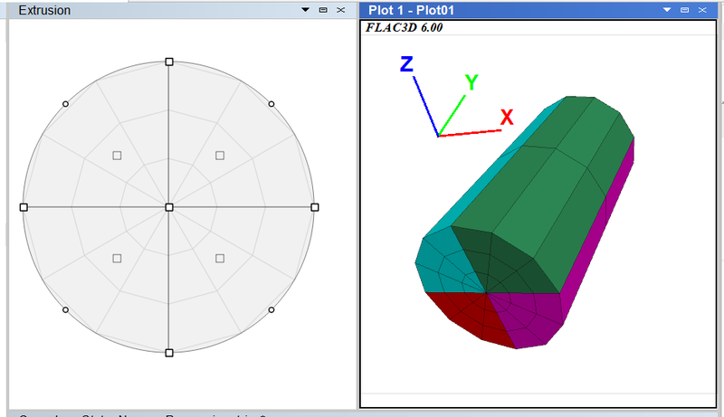
Next the State Record Pane is used to create a data file that recreates this result (the file is named cylinder.dat — called in the first line of the data file above). Next a FISH function that measures stress at the end of the cylinder and stores the result in a table is written and saved as measure.f3fis (this is called on the second line of the data file above and is shown at the end of this example, for reference).
With these two preliminaries in hand, the data file can be run, and the following is produced from the result table (see data file below):
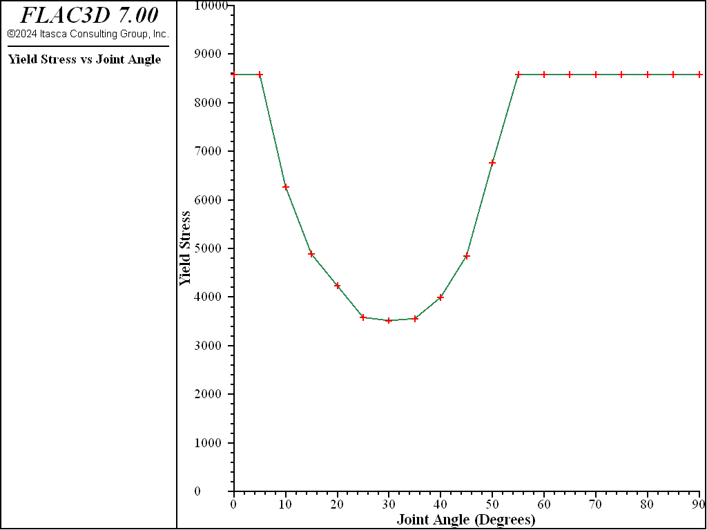
Note that in the actual verification problem the applied boundary conditions use a FISH servo to optimize convergence accuracy and the result is compared against an analytical solution calculated via FISH.
fish define measureStress(angle)
    ; Find list of grid points at y==0, using splitting and filtering
    local gplist = gp.list(gp.pos(::gp.list)->y == 0)
    ; Find unbalanced (reaction) force on those grid points, in y
    local force = -list.sum(gp.force.unbal(::gplist)->y)
    ; Convert force to stress, area of base is not quite a unit circle
    ;    due to linearization of the edge.
    local stress = force / 3.06147
    ; Store result in a table for later reference/plotting
    table('result',angle) = stress
end
| Was this helpful? ... | PFC © 2021, Itasca | Updated: Feb 25, 2024 |