
Double-Yield Model
Permanent volume changes caused by the application of isotropic pressure are taken into account in this model by including, in addition to the shear and tensile failure envelopes in the strain-softening/hardening model, a volumetric yield surface (or “cap”). For simplicity, the cap surface, defined by the “cap pressure” \(p_c >\) 0, is independent of shear stress; it consists of a vertical line on a plot of shear stress versus mean stress. The hardening behavior of the cap pressure is activated by volumetric plastic strain, and follows a piecewise-linear law prescribed in a user-supplied table. The tangential bulk and shear moduli evolve as plastic volumetric strain takes place according to a special law defined in terms of a factor, \(R\), assumed to be constant, and defined as the ratio of elastic bulk modulus to plastic bulk modulus.
Formulations
Only two additional material parameters and a table are required, in addition to those associated with the strain-softening model:
- the initial value of \(p_c\), which corresponds to the maximum mean pressure that the material has experienced in the past;
- the value of \(R\), greater than unity, which controls the slope of the stress-strain curve on volumetric unloading (the “swelling” line, in soil mechanics terms); and
- the table representation of the “hardening curve,” which relates cap pressure, \(p_c\), to plastic volume strain, \(e^{pv}\).
Hence, any laboratory-determined hardening behavior may be modeled within the constraints imposed by a two-parameter model.
Incremental Elastic Law
In the FLAC3D/3DEC implementation of this model, principal stresses \(\sigma_1\), \(\sigma_2\), \(\sigma_3\) are used. The principal stresses and principal directions are evaluated from the stress tensor components, and ordered so that (recall that compressive stresses are negative)
The corresponding principal strain increments \(\Delta e_{1}, \Delta e_{2}, \Delta e_{3}\) are decomposed:
where the superscripts \(e\) and \(p\) refer to elastic and plastic parts, respectively, and the plastic components are nonzero only during plastic flow. (Note that extensional strains are positive.) It is assumed that the plastic contributions of shear, tensile, and volumetric yielding are additive, so we may write
where the superscripts \(ps\), \(pt\), and \(pv\) stand for plastic shear, plastic tensile, and plastic volumetric strain. By convention, in this section, the symbol \(\Delta e\) is used to refer to the minus volumetric strain increment \((\Delta e_1 + \Delta e_2 + \Delta e_3)\) with plastic part \(\Delta e^p\) and elastic part \(\Delta e^e\). The symbol \(\Delta e^{pv}\) refers to minus the value of the plastic volumetric strain \((\Delta e_1^{pv} + \Delta e_2^{pv} + \Delta e_3^{pv})\).
The incremental expression of Hooke’s law in terms of principal stress and strain has the form
where \(\alpha_1 = K_c + 4G_c/3\), \(\alpha_2 = K_c-2G_c/3\), and \(K_c\) and \(G_c\) are the current tangential bulk and shear moduli defined according to the following considerations.
Consider an isotropic compression test with increasing pressure, \(p_c\). As the material becomes more compact, its plastic stiffness (\(d p_c / d e^{pv}\)) usually increases. It seems reasonable that the elastic stiffness will also increase, since the grains are being forced closer together. A simple rule is adopted in this model whereby, under general loading conditions, the incremental elastic stiffness, \(K_c\), is a constant factor, \(R\), multiplied by the current incremental plastic stiffness. The values of bulk and shear modulus, \(K\) and \(G\), supplied by the user are taken as upper limits to \(K_c\) and \(G_c\), and it is assumed that the ratio \(K_c/G_c\) remains constant and equal to \(K/G\). Using incremental notation, this law is defined by the relations
where the factor \(R\) is given, and \(\Delta p_c / \Delta e^{pv}\) is the current slope of the table of \(p_c\) values.
The type of behavior exhibited by the double-yield model is illustrated in Figure 1, which shows a nonlinear volumetric loading curve with several unloading excursions; these excursions are elastic, with slope related by \(R\) to the plastic stiffness at the point of unloading.
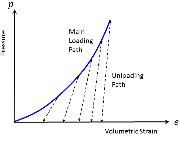
Figure 1: Elastic volumetric loading/unloading paths.
Yield and Potential Functions
The shear and tensile yield functions, referred to as \(f^s\) and \(f^t\), have the form
where
and \(\phi\) is the friction angle, \(c\) is the cohesion, and \(\sigma^t\) is the tensile strength.
The volumetric yield function \(f^v\) is defined as
where \(p_c\) is the cap pressure.
The shear potential function, \(g^s\), corresponds to a nonassociated flow rule; the tensile and volumetric potential functions, \(g^t\) and \(g^v\), correspond to associated laws. They have the form
where
and \(\psi\) is the dilation angle.
Hardening/Softening Parameters
The shear and volume yield surfaces can harden (or soften), and the tensile yield surface can soften, according to hardening rules that are specified by user-defined tables. Entry to the tables is by hardening parameters that record some measure of accumulated plastic strain. In shear and tension, the hardening parameter incremental forms are
where
\(\Delta e_j^{ps}, j\) = 1,3, and \(\Delta e_3^{pt}\) are plastic shear and tensile strain increments in the principal directions.
In the volumetric direction, the hardening parameter increment is
where \(\Delta e_j^{pv}, j\) = 1,3 are plastic volumetric strain increments in the principal directions.
These hardening parameters are used in the tables to determine new values of friction, cohesion, dilation, tensile strength, and cap pressure. The current bulk and shear moduli are also calculated from the table values as per Equations (5) and (6).
Plastic Corrections
Let the superscript \(I\) be used to represent the elastic guess obtained by adding to the old stresses \(\sigma_{ij}^O\), elastic increments computed using the total strain increments. In principal axes, we then have
In the FLAC3D/3DEC implementation, shear yield is detected if \(f^s(\sigma_1^I,\sigma_3^I) <\) 0, volumetric yield if \(f_v(\sigma_1^I,\sigma_2^I,\sigma_3^I) <\) 0, and tensile yield if \(f^t(\sigma_3^I) <\) 0. Corresponding plastic corrections are evaluated using the following techniques.
We first consider the case where tensile failure is not detected for the step, but both shear and volumetric yield conditions are exceeded. Using Equations (2) and (3), the principal strain increments may be expressed as
The flow rules for shear and volumetric yielding are
where \(i\) = 1,3. Using Equations (11) to (13), these expressions become, after differentiation:
and
Substituting in Equation (15), we obtain
With these expressions for the elastic strain increments, Hooke’s incremental equations yield (see Equation (4))
where \(\sigma_i^I\), \(i\) = 1,3, are the initial trial stresses in Equation (19), and \(\sigma_i^N = \sigma_i^O + \Delta \sigma_i\), \(i\) = 1,3 are the new principal stresses for the step.
To determine the multipliers \(\lambda^s\) and \(\lambda^v\), we require that if shear and volumetric yielding occur, the new stresses lie on both yield surfaces and we must have \(f^s(\sigma_1^N,\sigma_3^N)\) = 0 and \(f^{\sigma}(\sigma_1^N,\sigma_2^N,\sigma_3^N)\) =0. Substituting Equation (25) for \(\sigma_i,i\) = 1,3 in Equations (7) and (10), and solving for \(\lambda^s\), we obtain
Hence,
In these equations, the notation \(f^I\) stands for the function \(f\) evaluated for the initial trial stresses.
Equations (27) and (28) can now be used to evaluate the new stresses from Equation (26); these stresses simultaneously satisfy both yield conditions and both flow rules.
If the element is only yielding in shear, then
If the element is only yielding in volume, then
Equation (29) to (32) may be used in Equation (26), as appropriate, to compute new stresses.
We now consider the case where tensile failure is detected by the condition \(f^t(\sigma_3^I) <\) 0. If volumetric failure is not detected, we use the same technique and stress corrections as described in the Mohr-Coulomb model. If volumetric failure is detected in addition to tensile failure, then either \(f^s(\sigma_1^I,\sigma_3^I) \leq\) 0 or \(f^s(\sigma_1^I,\sigma_3^I) >\) 0. We begin by assuming that all three yield conditions are exceeded. We assume that the plastic contributions of shear, volumetric, and tensile yielding are additive:
The flow rule for tensile yielding has the form
Using Equation (8), these expressions become, after partial differentiation:
Using the same reasoning as above, and Equations (23) and (24) for the shear and volumetric flow rule, we obtain
The multipliers \(\lambda^s\), \(\lambda^v\), and \(\lambda^t\) are determined by solving the system of three equations, \(f^s (\sigma_1^N, \sigma_3^N)\) = 0, \(f^v (\sigma_1^N, \sigma_2^N, \sigma_3^N)\) = 0, and \(f^t (\sigma_3^N)\) = 0. This gives
Substitution of those expressions in Equation (36) yields
If only tensile and volumetric yield are detected, then \(\lambda^s\) = 0 in Equation (37). The constants \(\lambda^v\) and \(\lambda^t\) are determined by requiring that conditions \(f^v(\sigma_1^N,\sigma_2^N,\sigma_3^N)\) = 0 and \(f^t(\sigma_3^N)\) = 0 both be fulfilled. After some manipulation, we obtain
Substitution of those expressions in Equation (36) gives
Implementation Procedure
Hardening and softening behaviors for the cohesion, friction, and dilation in terms of the shear parameter \(e^{ps}\) (see Equation (15)) are provided by the user in the form of tables. Softening of the tensile strength is described in a similar manner using the parameter \(e^{pt}\) (see Equation (16)). In turn, the variation of cap pressure is specified in a table in terms of the parameter \(e^{pv}\) (see Equation (18)). Each table contains pairs of values: one for the parameter, and one for the corresponding property value. It is assumed that the property varies linearly between two consecutive parameter entries in the table.
In the implementation of the double-yield model in FLAC3D/3DEC, new stresses for the step are computed using the current values of the model properties. In this process, an elastic guess, \(\sigma_{ij}^I\), is first computed by adding to the old stress components, increments calculated by application of Hooke’s law to the total strain increment for the step. Principal stresses \(\sigma_1^I, \sigma_2^I, \sigma_3^I\), and corresponding principal directions, are calculated and ordered. If these stresses violate the composite yield criterion, corrections are applied to the elastic guess to give the new stress state. The stress tensor components in the system of reference axes are then calculated from the principal values by assuming that the principal directions have not been affected by the occurrence of a plastic correction.
Plastic strain increments are evaluated from Equations (23), (24), and (35), using relevant expressions of \(\lambda^s\), \(\lambda^t\) and \(\lambda^v\) for the mode of failure taking place. Zone hardening increments are then calculated as the surface average of values obtained from Equations (15), (18), and (16) for all triangles involved in the zone. The hardening parameters are updated, and new zone properties for cohesion, friction, dilation, tensile strength, and cap pressure are evaluated by linear interpolation in the tables. New elastic constants are derived from the cap pressure table using Equations (36). All these properties are stored for use in the next step. The hardening or softening lags one timestep behind the corresponding plastic deformation. In an explicit code, this error is small because the steps are small.
For a material with friction, the maximum value of the tensile strength is evaluated from \(c/\tan \phi\), using the new cohesion and friction angle. This value is retained by the code if it is smaller than the tensile strength updated from the table.
Choice of Volumetric Properties
The “hardening curve” and ratio, \(R\), of elastic bulk modulus to plastic bulk modulus are volumetric properties that may be derived from the results of a triaxial test in which axial stress and confining pressure, \(p\), are kept equal. This test (for which \(de^p = de^{pv}\)) is recommended because it is best to determine the parameters related to a particular mode of failure from a test that only involves that failure mode.
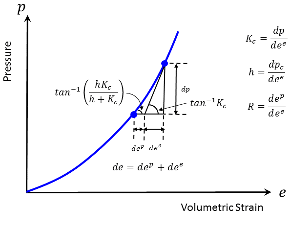
Figure 2: Isotropic consolidation test.
Consider the experimental graph of minus mean stress (pressure) versus minus volumetric strain for an increasing stress level with a small unloading excursion, obtained from such a test and presented in Figure 2. The volumetric strain increment \(de\) at a point of the main loading path (assuming that we are above any initial pre-consolidation stress level) is composed of an elastic part, \(de^e\), and a plastic part, \(de^p\). (Recall that, in this section, \(de\), \(de^e\), and \(de^p\) refer to minus the value of the volumetric strain.) The observed tangent modulus may be expressed as
where \(h\) is the plastic modulus, \(K_c\) is the elastic modulus, and, by definition:
With the preceding notation convention, the volumetric property, \(R\), may be defined as
and Equation (41) becomes
Expressing \(R\) from this relation, we obtain
Values for \(dp/de\) and \(K_c\) can be estimated from main loading and unloading increments on the graph. Hence, \(R\) can be calculated from Equation (44). Note that in the context of this model, the ratio \(R\) is assumed to be constant. Using \(K_c = Rh\) and \(h = dp_c/de^p\) in Equation (41), we can write, after some manipulation,
From this, it follows that values of \(p_c\) for a particular \(e^p\) can be obtained to the first approximation by multiplying the value \(p\) on the graph corresponding to \(e = e^p\) by the ratio \((1 + R)/R\). For example, if \(R\) = 5, then the graph curve must be scaled by a factor of 1.2 to convert it to table values, assuming no over-consolidation.
The double-yield model was initially developed to represent the behavior of mine backfill material, for which pre-consolidation pressures are low. The modified Cam-clay model is more applicable to soils such as soft clays for which pre-consolidation pressures can have a significant effect on material behavior.
Comparison of the Double-Yield and Modified Cam-Clay Model
In the double-yield model:
- Elastic moduli remain constant during elastic loading and unloading.
- Shear and tensile failure are not coupled to plastic volumetric change, due to volumetric yielding. The shear yield function corresponds to the Mohr-Coulomb criterion, and the tensile yield is evaluated based on a tensile strength.
- Material hardening or softening, upon shear or tensile failure, is defined by tables relating friction angle and cohesion to plastic shear strain, and tensile strength to plastic tensile strain.
- Volumetric yielding occurs; the isotropic stress at which yield occurs (the cap pressure) is not influenced by the amount of shear or tensile plastic deformation, but it increases (or hardens) with volumetric plastic strain.
- A tensile strength limit and tensile softening can be defined.
In the modified Cam-clay model:
- The elastic deformation is nonlinear, with the elastic moduli depending on mean stress.
- hear failure is affected by the occurrence of plastic volumetric deformation: the material can harden or soften depending on the degree of pre-consolidation.
- As shear loading increases, the material evolves toward a critical state at which unlimited shear strain occurs with no accompanying change in specific volume or stress.
- There is no resistance to tensile mean stress.
double-yield model properties
Use the following keywords with the zone property (FLAC3D) or block zone property (3DEC) command to set these properties of the double-yield model.
- double-yield
- bulk-maximum f
maximum elastic bulk modulus, \(K_{max}\)
- cohesion f
cohesion, \(c\)
- friction f
angle of internal friction, \(\phi\)
- multiplier f
multiplier on current plastic cap modulus to give elastic bulk and shear moduli, \(R\). The default is 5.0.
- pressure-cap f
current intersection of volumetric yield surface with pressure axis, \(p_c\)
- shear-maximum f
maximum elastic shear modulus, \(G_{max}\)
- flag-brittle b (a)
If true, the tension limit is set to 0 in the event of tensile failure. The default is false.
- table-cohesion s (a)
name of the table relating cohesion to plastic shear strain. The default is a null string.
- table-dilation s (a)
name of the table relating dilation angle to plastic shear strain. The default is a null string.
- table-friction s (a)
name of the table relating friction angle to plastic shear strain. The default is a null string.
- table-pressure-cap s (a)
name of the table relating cap pressure to plastic volume strain. The default is a null string.
- table-tension s (a)
name of the table relating tensile limit to plastic tensile strain. The default is a null string.
- bulk f (r)
current elastic bulk modulus, \(K\)
- poisson f (r)
current Poisson’s ratio, \(\nu\)
- shear f (r)
current elastic shear modulus, \(G\)
- strain-shear-plastic f (r)
accumulated plastic shear strain
- strain-tensile-plastic f (r)
accumulated plastic tensile strain
- strain-volumetric-plastic f (r)
accumulated plastic volumetric strain
- young f (r)
current elastic Young’s modulus, \(E\)
Key
- (a) Advanced property.
- This property has a default value; simpler applications of the model do not need to provide a value for it.
- (r) Read-only property.
- This property cannot be set by the user. Instead, it can be listed, plotted, or accessed through FISH.
Notes
- If table-pressure-cap is not assigned, the model moduli will be constant, so that \(K\) = \(K_{max}\) and \(G\) = \(G_{max}\). In any case, \(K_{max}\) and \(G_{max}\) are upper limits of moduli.
- The tension cut-off is \({\sigma}^t = min({\sigma}^t, c/\tan \phi)\).
- The tension table and flag-brittle should not be active at the same time.
| Was this helpful? ... | PFC © 2021, Itasca | Updated: Feb 25, 2024 |