
Wave Propagation in Particle Assemblies
Problem Statement
Note
The project file for this example may be viewed/run in PFC.[1] The data files used are shown at the end of this example.
Wave propagation through an assembly of discrete bodies is, in general, dispersive. That is, the apparent wave velocity depends on wavelength, particularly for wavelengths that approach the mean particle size. For longer wavelengths, the propagation resembles that in a continuous elastic medium without an internal length scale. The following example illustrates plane wave propagation through a one-dimensional “bar” composed of a string of 50 particles bonded together. The right-hand end of the bar is free, and the left-hand end is a “quiet boundary” that absorbs any incident waveform. An input pulse is also injected at the left-hand boundary. In order to absorb waves, the left-hand boundary is terminated with the acoustic impedance of the medium, \(Cρ\), where \(C\) is the wave speed and \(ρ\) is the density. This is discussed in more detail below.
In order to establish an equivalence between continuum parameters and particle parameters, we assume that the particle string is equivalent to a continuous, elastic bar. The equivalent bar has a circular cross-section of radius \(R\) in 3D, and a rectangular cross-section of height \(2R\) and unit thickness in 2D, where \(R\) is the particle radius. In the axial direction, each particle corresponds to a solid cylinder of length \(2R\) in 3D and a solid rectangular prism of length \(2R\) in 2D. The Young’s modulus is expressed as
where \(F\) is the contact force and \(u\) is the contact displacement. Noting that \(F/u = k_n\)\(/2\) for a contact (where \(k_n\) is the normal stiffness, defined for a particle), we obtain
The equivalent particle density, \(u̇\), is obtained by equating the particle mass to the mass of the equivalent bar element, which leads to
For longitudinal waves,
Substituting from Equation (2) and rearranging:
Given the wave speed and density of a bar, the necessary particle stiffness and density are then obtained from Equation (5) and Equation (3), respectively.
For a plane wave in a continuous medium, stress is related to particle velocity, \(u̇\), by the acoustic impedance, \(Cρ\):
If this relation is enforced at an artificial boundary, then the boundary absorbs all incident dynamic energy (because the constitutive behavior of the boundary is identical to that of an infinite continuation of the bar). Replacing \(σ\) with {\(F/2R\) in 2D, \(F/πR²\) in 3D} in Equation (6), we obtain a relation between boundary force, \(F\), and velocity:
To inject a given velocity pulse, \(U̇(t)\), we superimpose double the equivalent force at the boundary (in which the factor of two accounts for the equal partition of energy between the “real” bar and the “fictitious” bar, represented by the terminating impedance):
Finally, to ensure symmetry between the real and fictitious parts, the mass of the boundary particle is set to half the mass of the others.
Numerical Model
The data files “wave_propagation.dat (2D)” and “wave_propagation.dat (3D)” simulate wave propagation in a bar made up of a row of 50 bonded particles in 2D and 3D, respectively. The time history of the input pulse is
where \(A\) is the amplitude of the pulse and \(f\) is the frequency. The duration of the pulse is 1\(/f\), and \(U̇\) (the velocity applied to the PFC model) is set to zero after the duration of the pulse. Parameters \(R, ρ, C, f\), and \(A\) are set in the initial section of “wave_propagation.dat (2D)” and “wave_propagation.dat (3D)”“.
When the data files are executed with PFC, the time histories reproduced in Figures #ver-wavp-wave2 (2D model)
and 2 (3D model) are generated. The three curves correspond to the left-hand end, the middle, and the right-hand end of the bar. The time interval between successive peaks is found to be 0.25 second, which verifies that the wave velocity is 100 m/sec, as intended (since the distance between measurement points is 25 m). The time history for the right-hand end shows a peak velocity of double the input velocity, which is the correct response for reflection at a free surface. The fourth peak corresponds to the reflected wave traveling toward the left boundary. The wave “passes through” the left boundary (fifth peak); the absence of further pulses indicates that the quiet boundary condition has absorbed the incident energy. The slight oscillations at the trailing edges of the main pulses are consequences of the discrete nature of the medium. If the wavelength were to be reduced, the oscillations would increase relative to the amplitude of the main pulse. This is not a numerical artifact; it is the correct response of a discrete medium.
The reference [Lysmer1969] should be consulted for more details.
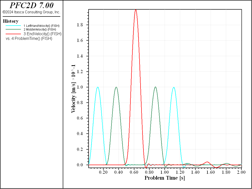
Figure 1: Velocity histories at three points in the bar: the “input” end, the middle, and the free end (2D model).
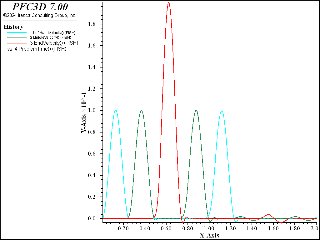
Figure 2: Velocity histories at three points in the bar: the “input” end, the middle, and the free end (3D model).
Reference
| [Lysmer1969] | Lysmer, J., and R. L. Kuhlemeyer. “Finite Dynamic Model for Infinite Media,” J. Eng. Mech., 95(EM4), 859-877 (1969). |
Data Files
wave_propagation.dat (3D)
model new
model large-strain on
model title 'Wave Propagation in Particle Assemblies (3D)'

fish define makeTheBar
  ; given parameters ...
  NumBalls = 50
  BallRadius = 0.5
  BarDensity = 1000.0
  WaveSpeed = 100.0
  Freq = 4.0 ; frequency of the pulse
  Amplitude = 0.1 ; m/sec peak pulse velocity
  ; derived parameters ...
  BallDensity = 3.0 * BarDensity / 2.0
  HalfDensity = BallDensity / 2.0
  ContactStiff = WaveSpeed*WaveSpeed * math.pi * BarDensity * BallRadius
  Impedance = math.pi * BallRadius*BallRadius * WaveSpeed * BarDensity
  ; create the assembly
  XBall = 0.0
  loop nn (1,NumBalls)
    command
      ball create id=[nn] rad=[BallRadius] position-x=[XBall]
    endcommand
    XBall = XBall + 2.0 * BallRadius
  endLoop
  LHAddress  = ball.find(1)
  MidAddress = ball.find(NumBalls/2)
  EndAddress = ball.find(NumBalls)
  check_endvel = 0.0
end

fish define Wave ; input waveform
  if mech.time.total > 1.0 / Freq
    Wave = 0.0
  else
    Wave = ...
       (1.0 - math.cos(2.0*math.pi*Freq*mech.time.total)) * Amplitude / 2.0
  endif
end

fish define InputWave
  whilestepping
  ball.force.app(LHAddress,1) = ...
     Impedance * (2.0 * Wave - ball.vel(LHAddress,1))
end

fish define LeftHandVelocity
  LeftHandVelocity = ball.vel(LHAddress,1)
  MiddleVelocity   = ball.vel(MidAddress,1)
  EndVelocity      = ball.vel(EndAddress,1)
  ProblemTime = mech.time.total
  check_endvel = math.max(check_endvel,EndVelocity)
end

;---------------------------------------------------------------
program echo off
model domain extent -2.0 52.0 -2.0 2.0 -2.0 2.0 cond d d d
contact cmat default model LinearCBond
[MakeTheBar]
program echo=on
ball attribute density [BallDensity]
ball attribute density [HalfDensity] range id=1
ball property 'kn' [ContactStiff]
model clean
contact method bond

ball fix velocity-y velocity-z spin-x spin-y spin-z
history interval 1
fish history LeftHandVelocity
fish history MiddleVelocity
fish history EndVelocity
fish history ProblemTime
model solve elastic only time-total 2.0
model save 'wave-final'
program return
wave_propagation.dat (2D)
model new
model large-strain on
model title 'Wave Propagation in Particle Assemblies (2D)'

fish define makeTheBar
  ; given parameters ...
  NumBalls = 50
  BallRadius = 0.5
  BarDensity = 1000.0
  WaveSpeed = 100.0
  Freq = 4.0 ; frequency of the pulse
  Amplitude = 0.1 ; m/sec peak pulse velocity
  ; derived parameters ...
  BallDensity = 4.0*BarDensity / math.pi
  HalfDensity = BallDensity / 2.0
  ContactStiff = 2.0*WaveSpeed^2 * BarDensity
  Impedance = 2.0*BallRadius * WaveSpeed * BarDensity
  ; create the assembly
  XBall = 0.0
  command
    model domain extent -2.0 52.0 -2.0 2.0 cond d d
  endcommand
  loop nn (1,NumBalls)
    command
      ball create id=[nn] rad=[BallRadius] position-x=[XBall]
    endcommand
    XBall = XBall + 2.0 * BallRadius
  endLoop
  LHAddress = ball.find(1)
  MidAddress = ball.find(NumBalls/2)
  EndAddress = ball.find(NumBalls)
  check_endvel = 0.0
end

fish define Wave ; input waveform
  if mech.time.total > 1.0 / Freq
    Wave = 0.0
  else
    Wave = ...
       (1.0 - math.cos(2.0*math.pi*Freq*mech.time.total)) * Amplitude / 2.0
  endif
end

fish define InputWave
  whilestepping
  ball.force.app(LHAddress,1) = ...
     Impedance * (2.0 * Wave - ball.vel(LHAddress,1))
end

fish define LeftHandVelocity
  LeftHandVelocity = ball.vel(LHAddress,1)
  MiddleVelocity = ball.vel(MidAddress,1)
  EndVelocity = ball.vel(EndAddress,1)
  ProblemTime = mech.time.total
  check_endvel = math.max(check_endvel,EndVelocity)
end

;---------------------------------------------------------------
program echo off
[MakeTheBar]
contact cmat default model linearcbond
program echo=on
ball attribute density [BallDensity]
ball attribute density [HalfDensity] range id=1
ball property 'kn' [ContactStiff]
model clean
contact method bond gap 0.0
ball fix velocity-y spin
history interval 1
fish history LeftHandVelocity
fish history MiddleVelocity
fish history EndVelocity
fish history ProblemTime
model solve elastic only age 2.0
program return
Endnotes
| [1] | To view this project in PFC, use the program menu.
⮡ PFC |
⇐ Hertz Contact Model: Complex Loading Paths | Rolling Resistance Linear Contact Model: Single Ball on a Flat Surface ⇒
| Was this helpful? ... | PFC © 2021, Itasca | Updated: Feb 25, 2024 |