
Rolling Resistance Linear Contact Model: Single Ball on a Flat Surface
Problem Statement
Note
The project file for this example may be viewed/run in PFC.[1] The data files used are shown at the end of this example.
The rolling resistance linear contact model is exercised with a simple system consisting of one ball initially at rest under gravity on a flat surface. The ball is then given a non-zero initial velocity in the direction parallel to the surface, and the model is cycled for a desired mechanical age. This setup is similar to verification problems discussed in [Ai2011] and [Wensrich2012]. Five cases are simulated:
- in the first 3 cases, gravity is acting perpendicular to the surface (i.e. the surface is horizontal), and the contact model properties are varied to demonstrate the behavior of the contact model;
- In the last 2 cases, gravity is rotated (i.e. the surface is inclined), and the influence of the rolling resistance coefficient is discussed.
In all cases, the model is cycled until a target mechanical time of 1.5 seconds is met.
PFC2D model
The system consists in a single ball put at rest on a flat surface under gravity. The initial state is built using the file make_system.dat, as described below.
First, the system is constructed and cycled to equilibrium using the following commands:
; define domain extent and boundary conditions
model domain extent -1.0 1.0 -1e-1 2e-1 condition destroy

; set the defaults slots of the CMAT to use the rrlinear contact model
contact cmat default model rrlinear ...
                            method deformability emod 1e7 kratio 1.0 ...
                            property dp_nratio 0.2 dp_mode 3

; create the system and settle under gravity
wall generate plane
ball create radius 5e-3 position-y 5e-3
ball attribute density 2500.0
model gravity 9.81
model large-strain on
model solve
Note that the default slots of the CMAT are filled with the rolling resistance linear contact model.
Before performing the different test cases, history monitoring is set up and the ball is given an initial x-velocity of 1 m/s.
; set up history monitoring
model mechanical time-total 0.0
model orientation-tracking on
model energy mechanical on
history interval  1
model history name "1" mechanical time-total
model history name "2" mechanical energy energy-kinetic
model history name "3" mechanical energy energy-slip
model history name "4" mechanical energy energy-rrslip
model history name "5" mechanical energy energy-dashpot
model history name "6" mechanical energy energy-strain
model history name "7" mechanical energy energy-rrstrain
ball history name "11" position-x id 1
ball history name "12" spin id 1
ball history name "13" velocity-x id 1
ball attribute velocity-x 1.0
model save 'system-ini'
program return
The initial system is shown in Fig. 1.
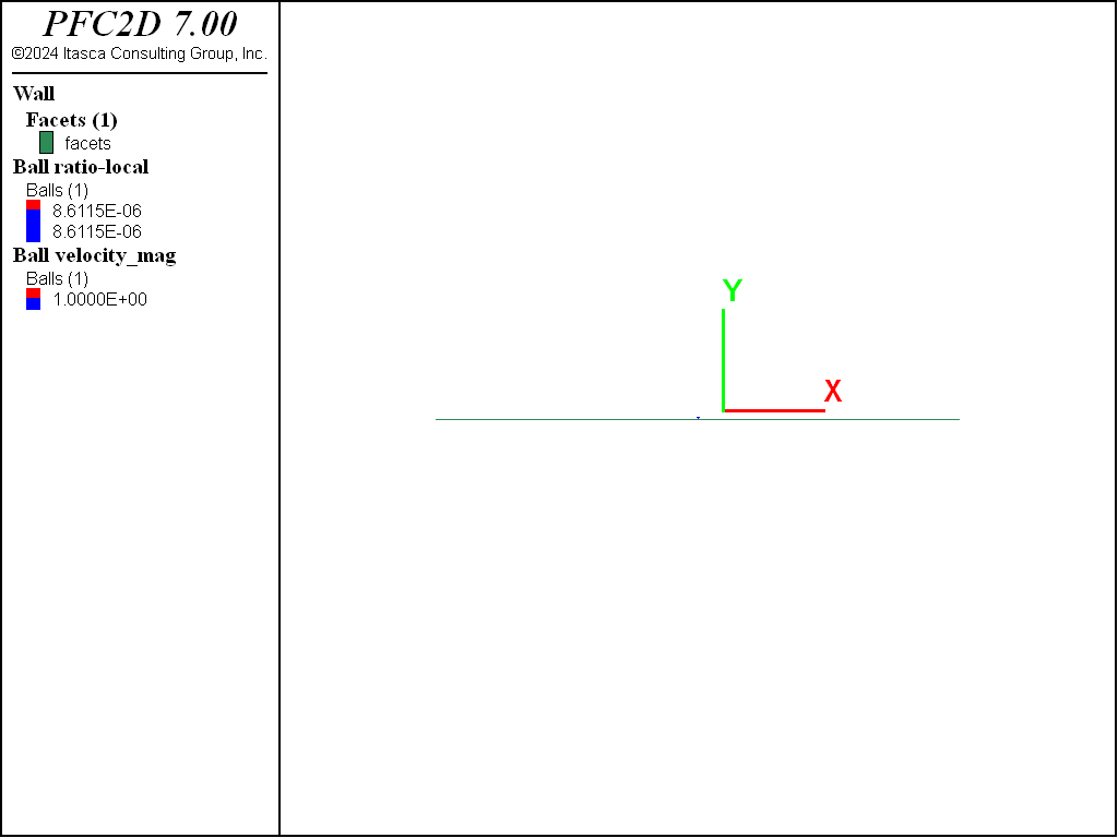
Figure 1: The initial system.
Horizontal Surface
Three simulations are performed with a horizontal surface, with varying values of the friction and rolling friction coefficients.
In the first case, the rolling friction coefficient is kept to zero, while a non-zero friction coefficient is set (\(\mu = 0.8\)). The behavior is therefore identical to that of a linear contact model under the same loading conditions. Fig. 2 illustrates the motion of the ball. It shows the histories of the x-position (top-left corner), x-velocity (top-right corner), angular velocity (bottom-left corner), as well as the histories of the kinetic energy and of the energy dissipated by frictional work (bottom-right) corner against mechanical age. Because the input translational velocity is large, friction is instantaneously fully mobilized (at the first timestep). The resulting torque causes the ball to rotate, while the kinetic energy is partially dissipated by frictional work and partially transfered to the rotational degree of freedom. After a short deceleration phase, the ball exhibits a constant x-velocity and a constant spin. During this phase, energy is no longer dissipated and the ball finally reaches the domain boundary.
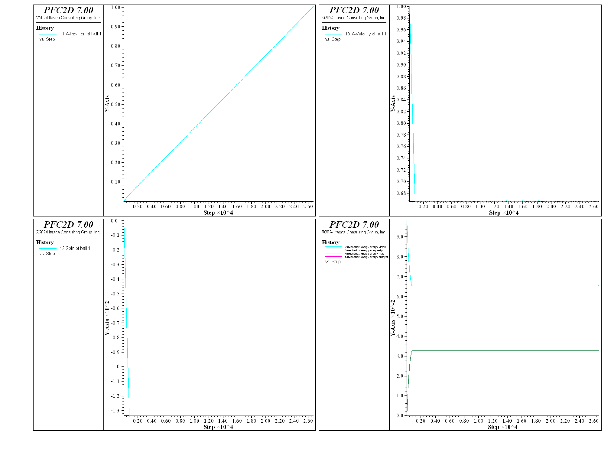
Figure 2: Histories monitored during the simulation, versus mechanical age (\(\mu = 0.8\), \(\mu_r = 0.0\)). Top-left: x-position, top-right: x-velocity, bottom-left: spin, and bottom-left: energies.
The simulation is repeated with a non-zero value of the rolling friction coefficient (\(\mu_r = 0.1\)). In this case (see Fig. 3), the rolling resistance mechanism seems at first glance able to dissipate energy until the ball reaches a final stable position.
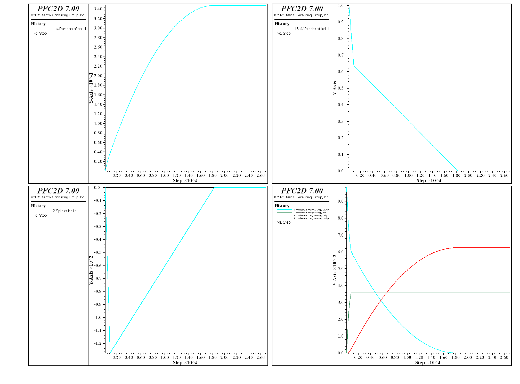
Figure 3: Histories monitored during the simulation, versus mechanical age (\(\mu = 0.8\), \(\mu_r = 0.1\)). Top-left: x-position, top-right: x-velocity, bottom-left: spin, and bottom-left: energies.
However, a closer look at the histories (Fig. 4) shows that the ball keeps oscillating around a constant position. This is due to the fact that neither the friction or rolling friction are fully mobilized at this stage, therefore the system lacks an additional damping mechanism to get rid of the remaining kinetic energy.
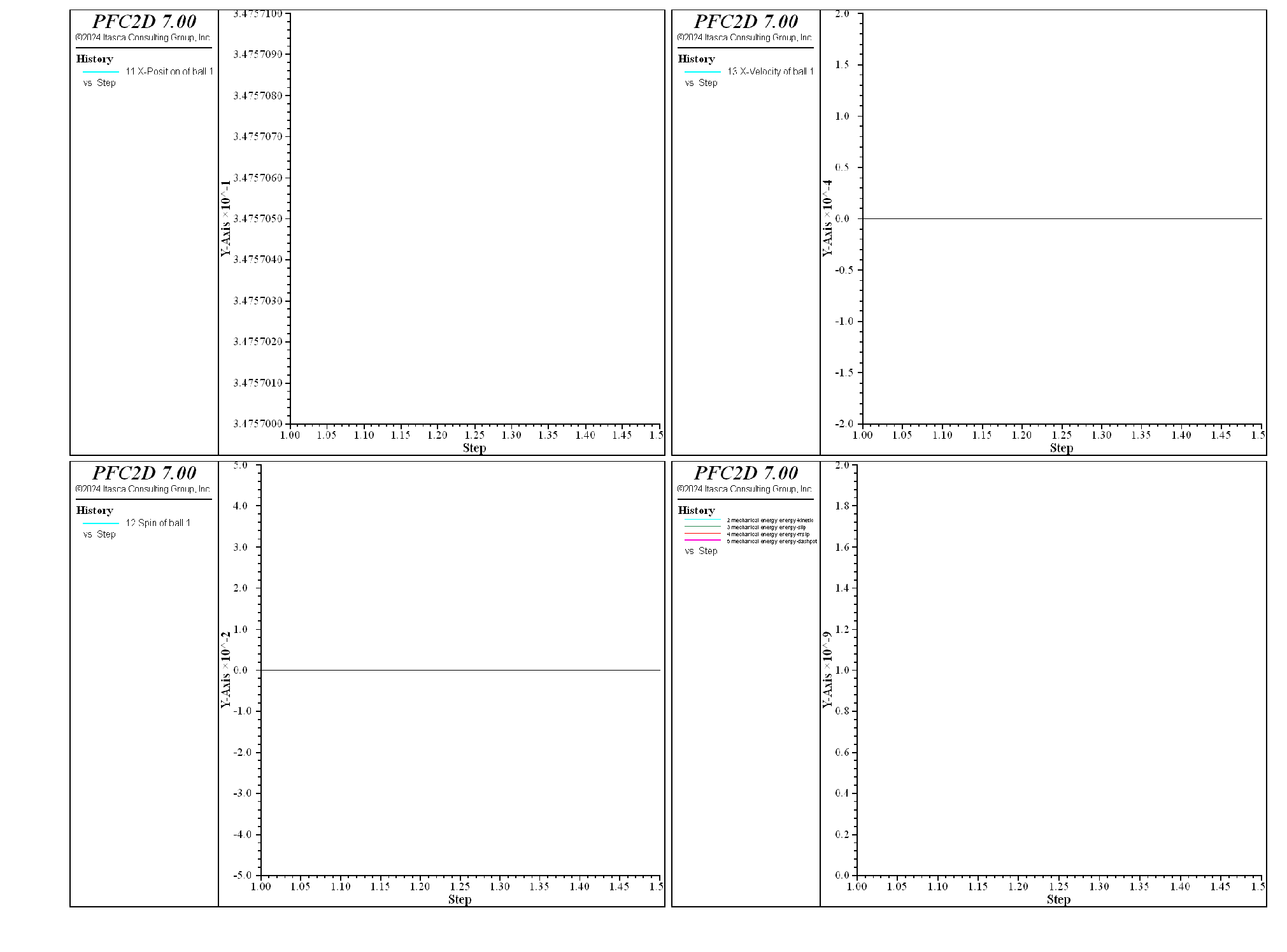
Figure 4: Histories monitored during the simulation, versus mechanical age (\(\mu = 0.8\), \(\mu_r = 0.1\)). Close view to the values between 1.0 and 1.5 seconds. Top-left: x-position, top-right: x-velocity, bottom-left: spin, and bottom-left: energies.
The same simulation is now repeated with a non-zero value of the critical damping ratio in the shear direction (\(\beta_s = 0.2\)). In this case (see Fig. 5), a very similar behavior is observed, where the rolling resistance mechanism is able to dissipate most of the energy, and viscous damping also dissipates energy, sufficiently to allow the ball to reach a final stable position (Fig. 6). It is worth noting that the stable final x-position is close, although slightly lower, than the value around which the system oscillates around without shear viscous damping (0.34756m compared to 0.34757m).
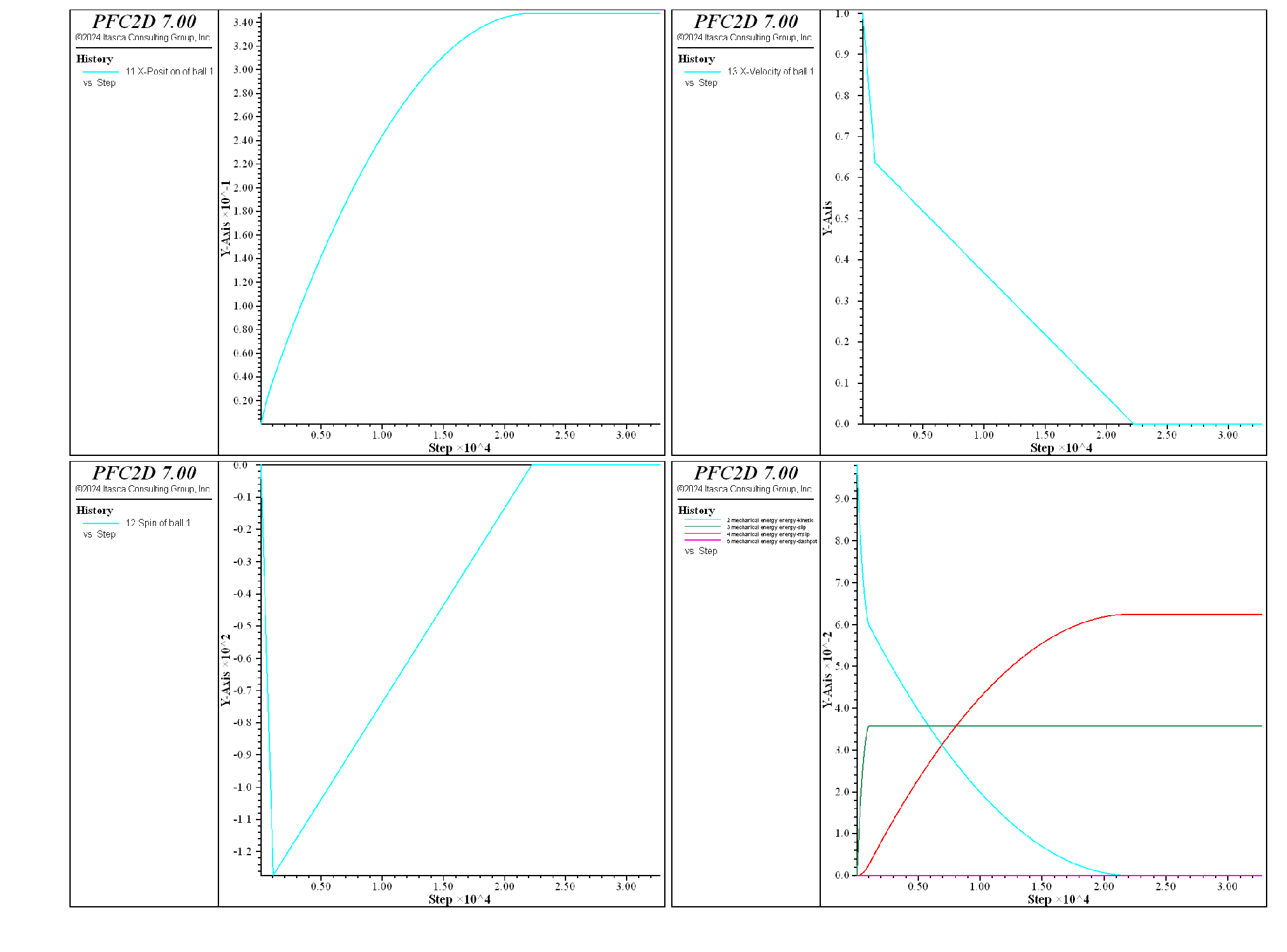
Figure 5: Histories monitored during the simulation, versus mechanical age (\(\mu = 0.8\), \(\mu_r = 0.1\), \(\beta_s = 0.2\)). Top-left: x-position, top-right: x-velocity, bottom-left: spin, and bottom-left: energies.
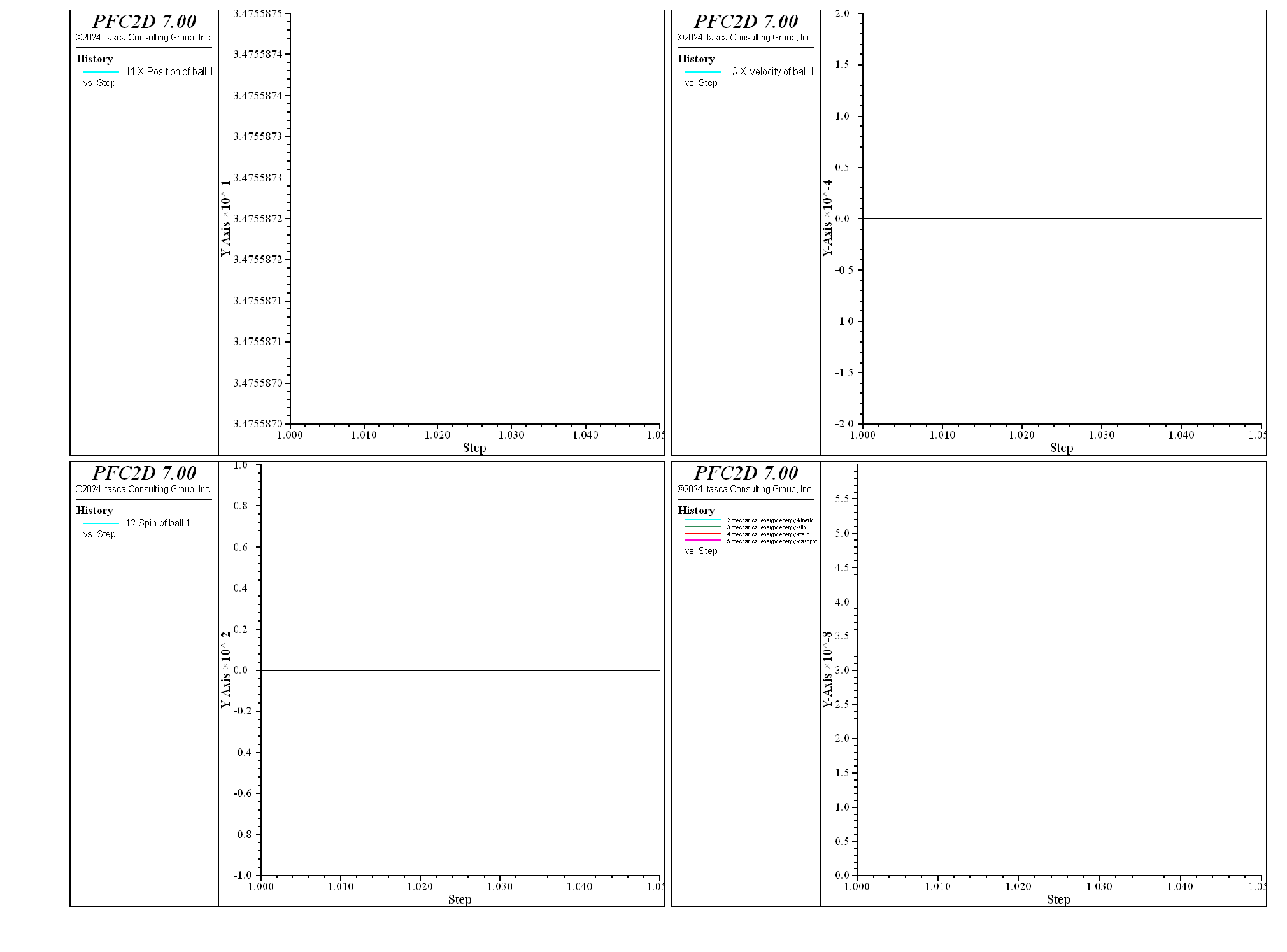
Figure 6: Histories monitored during the simulation, versus mechanical age (\(\mu = 0.8\), \(\mu_r = 0.1\), \(\beta_s = 0.2\)). Close view to the values between 1.0 and 1.5 seconds. Top-left: x-position, top-right: x-velocity, bottom-left: spin, and bottom-left: energies.
Inclined Surface
The simulation is performed two more times with gravity rotated in order to model a ball initially going up a slope, with an inclination angle \(\alpha=10^{\circ}\).
For the first case \(\mu = 0.8\), \(\mu_r = 0.1\) and \(\beta_s = 0.2\). With these parameters (see Fig. 7), the ball travels to a maximum distance, then starts rolling backward on the slope under the action of gravity. The small amount of rolling resistance is not sufficient to counterbalance the torque the ball is subjected to, and the ball accelerates downward.
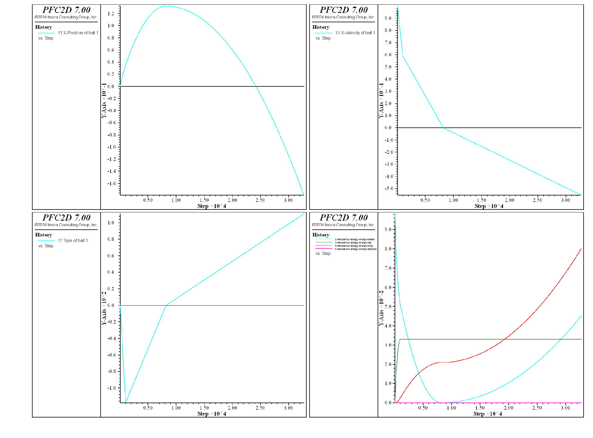
Figure 7: Histories monitored during the simulation, versus mechanical age (inclined slope: \(\alpha=10^{\circ}\), \(\mu = 0.8\), \(\mu_r = 0.1\), \(\beta_s = 0.2\)). Top-left: x-position, top-right: x-velocity, bottom-left: spin, and bottom-left: energies.
In the second case, the rolling friction coefficient is set to \(\mu_r = \tan \alpha\). The torque applied to the ball by the rolling resistance mechanism is now sufficient to counterbalance the torque the ball is subjected to due to gravitational loading ([Ai2011]), and the ball is prevented from moving downward (Fig. 8). Note that the final travelled distance decreases slightly. It would reach a finite final value should the system be cycled for a sufficient mechanical time.
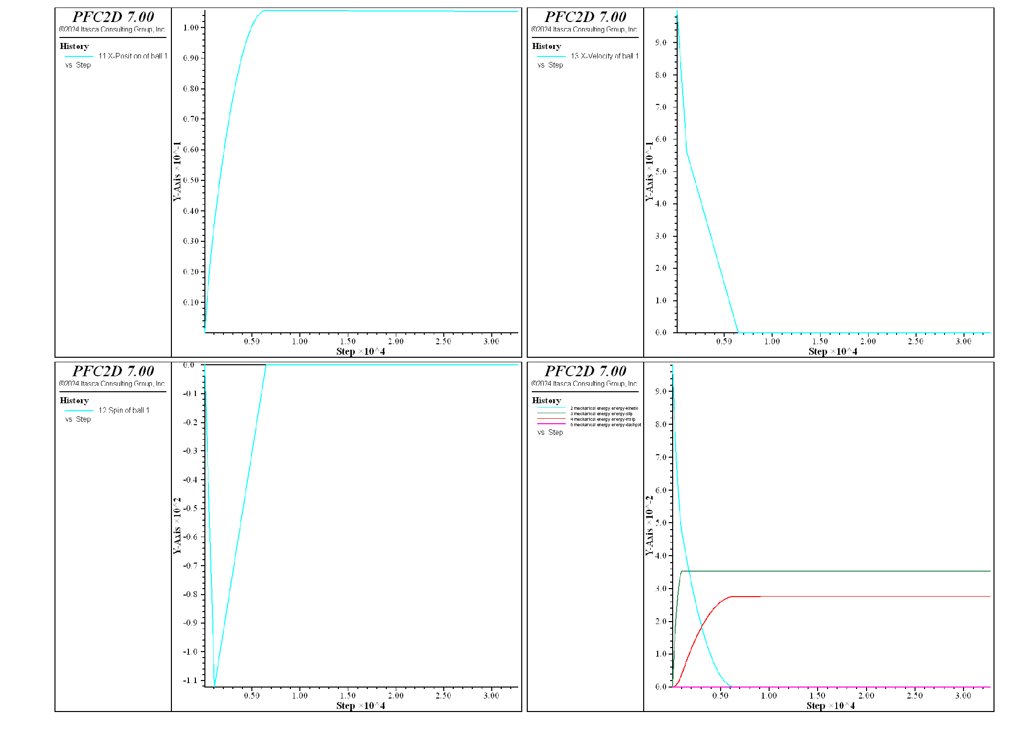
Figure 8: Histories monitored during the simulation, versus mechanical age (inclined slope: \(\alpha=10^{\circ}\), \(\mu = 0.8\), \(\mu_r = \tan \alpha\), \(\beta_s = 0.2\)). Top-left: x-position, top-right: x-velocity, bottom-left: spin, and bottom-left: energies.
Discussion
In this example, the rolling resistance linear contact model is exercised with a simple system consisting of one ball initially at rest under gravity on a flat surface. The ball is then given a non-zero initial velocity in the direction parallel to the surface, and the model is cycled for a desired mechanical age. The direction of gravitational acceleration is set perpendicular to the surface to simulate an horizontal surface, or at an angle to simulate an inclined surface. The result show that the rolling resistance mechanism is necessary to prevent the ball from rolling up to the domain boundary when the surface is horizontal. A small amount of shear viscous damping is also necessary to damp oscillations around the final position. In the case of an inclined plane, the ball decelerates under the action of gravity, and reaches a final position if the rolling friction coefficient is larger than the tangent of the inclination angle. Otherwise, the ball reaches a maximal height, then rolls back down the inclined surface. These results are in agreement with the results discussed in [Ai2011].
Data Files
make_system.dat (2D)
;===========================================================================
; fname: make_system.dat (2D)
;===========================================================================
model new
model title ...
'Rolling Resistance Linear Contact Model: Single Ball on a Flat Surface'

; excerpt-izrw-start
; define domain extent and boundary conditions
model domain extent -1.0 1.0 -1e-1 2e-1 condition destroy

; set the defaults slots of the CMAT to use the rrlinear contact model
contact cmat default model rrlinear ...
                            method deformability emod 1e7 kratio 1.0 ...
                            property dp_nratio 0.2 dp_mode 3

; create the system and settle under gravity
wall generate plane
ball create radius 5e-3 position-y 5e-3
ball attribute density 2500.0
model gravity 9.81
model large-strain on
model solve
; excerpt-izrw-end

; excerpt-ptwa-start
; set up history monitoring
model mechanical time-total 0.0
model orientation-tracking on
model energy mechanical on
history interval  1
model history name "1" mechanical time-total
model history name "2" mechanical energy energy-kinetic
model history name "3" mechanical energy energy-slip
model history name "4" mechanical energy energy-rrslip
model history name "5" mechanical energy energy-dashpot
model history name "6" mechanical energy energy-strain
model history name "7" mechanical energy energy-rrstrain
ball history name "11" position-x id 1
ball history name "12" spin id 1
ball history name "13" velocity-x id 1
ball attribute velocity-x 1.0
model save 'system-ini'
program return
; excerpt-ptwa-end
;===========================================================================
; eof: make_system.dat (2D)
test_system.dat (2D)
;===========================================================================
; fname: test_system.p2dat
;===========================================================================

; CASE HORIZONTAL-0: no rolling friction
model restore 'system-ini'
contact property fric 0.8
model solve time 1.5
model save 'final-horizontal-0.sav'

; CASE HORIZONTAL-1: friction and rolling friction
model restore 'system-ini'
contact property fric 0.8 rr_fric 0.1
model solve time 1.5
model save 'final-horizontal-1.sav'

; CASE HORIZONTAL-2: friction, rolling friction and damping
model restore 'system-ini'
contact property fric 0.8 rr_fric 0.1 dp_sratio 0.2
model solve time 1.5
model save 'final-horizontal-2.sav'

; CASE INCLINED-1: rolling friction below tangent of the slope inclination
model restore 'system-ini'
[theta = math.degrad*10.0]
model gravity [-9.81*math.sin(theta)] [-9.81*math.cos(theta)]
contact property fric 0.8 rr_fric 0.1 dp_sratio 0.2
model solve time 1.5
model save 'final-inclined-1.sav'

; CASE INCLINED-2: rolling friction equal to tangent of the slope inclination
model restore 'system-ini'
[theta = math.degrad*10.0]
model gravity [-9.81*math.sin(theta)] [-9.81*math.cos(theta)]
contact property fric 0.8 rr_fric [math.tan(theta)] dp_sratio 0.2
model solve time 1.5
model save 'final-inclined-2.sav'
program return
;=============================================================================
; eof: test_system.p2dat
Endnotes
| [1] | To view this project in PFC, use the program menu.
⮡ PFC |
| Was this helpful? ... | PFC © 2021, Itasca | Updated: Feb 25, 2024 |