Continuously Yielding Joint Model In 3DEC
Background
Numerical modeling of practical problems may take joints through rather complex load paths. Empirical models developed to fit laboratory tests only provide responses to simple loading conditions. More general situations require either interpolation between curves or other arbitrary assumptions. The continuously yielding joint model, proposed by Cundall and Hart (1984), is intended to simulate, in a simple fashion, the internal mechanism of progressive damage of joints under shear. The model also provides continuous hysteretic damping for dynamic simulations by using a “bounding surface” concept similar to that proposed by Dafalias and Herrmann (1982) for soils. An application of the model to study rock-fault instability induced by seismic events is reported by Cundall and Lemos (1990).
Formulation
The continuously yielding model is considered more “realistic” than the standard Mohr-Coulomb joint model in that the continuously yielding model attempts to account for some nonlinear behavior observed in physical tests, such as: joint shearing damage, normal stiffness dependence on normal stress, and decrease in dilation angle with plastic shear displacement. The essential features of the continuously yielding model include the following.
- The curve of shear stress/shear displacement is always tending toward a “target” shear strength for the joint (i.e., the instantaneous gradient of the curve depends directly on the difference between strength and stress).
- The target shear strength decreases continuously as a function of accumulated plastic displacement (a measure of damage).
- Dilation angle is taken as the difference between the apparent friction angle (determined by the current shear stress and normal stress) and the residual friction angle.
As a consequence of these assumptions, the model exhibits, automatically, the commonly observed peak/residual behavior of rock joints. Also, hysteresis is displayed for unloading and reloading cycles of all strain levels, no matter how small.
The model is described as follows. The response to normal loading is expressed incrementally as
where the normal stiffness, \(k_n\), is given by
representing the observed increase of stiffness with normal stress, where an and en are model parameters. In general, zero tensile strength is assumed.
For shear loading, the model displays irreversible nonlinear behavior from the onset of shearing. Figure 1 shows a typical stress-displ cement curve for monotonic loading under constant normal stress. The shear stress increment is calculated as
where the shear stiffness, \(k_s\) , can also be taken as a function of normal stress. For example,
The stiffness functions defined by Equation (2) and Equation (4) are the simplest functions consistent with the experimental data. More complex functions (such as hyperbolic laws) may be substituted, if desired.

Figure 1: Continuously yielding joint model: shear stress-displacement curve and bounding shear strength
The tangent modulus is governed in Equation (3) by the factor \(F\), which depends on the distance from the actual stress curve to the target or bounding strength curve, \(\tau_m\), as shown in Figure 1.
The factor \(r\), which is initially zero, is intended to restore the elastic stiffness immediately after a load reversal — that is, \(r\) is set to \(\tau/\tau_m\) (and, therefore, \(F\) to 1) whenever \(\rm{sgn}(Δu_s)\) is not equal to \(\rm{sgn}(Δu^{(old)}_s)\). In practice, \(r\) is limited to 0.75 in order to avoid numerical noise when the shear stress is approximately equal to the bounding strength. The bounding strength is given by
The parameter \(\phi_m\) can be understood as the friction angle that would apply if the joint were to dilate at the maximum dilation angle. As damage accumulates, this angle is continuously reduced according to the equation
where the plastic displacement increment is defined as
and \(\phi\) is the basic friction angle of the rock surfaces. \(R\) is a material parameter (with dimension of length) that expresses the joint roughness.
\(\phi_m\) can also be thought of as the effective friction angle that would apply if no damage were done (i.e., if no asperities were sheared off). However, before the corresponding strength can be mobilized some shear displacement is necessary, which reduces \(\phi_m\).
The parameter \(R\), which has the dimension of length, controls the rate at which \(\phi_m\) decreases with plastic shear displacement. A small value of \(R\) causes \(\phi_m\) to decrease rapidly. A large value of \(R\) leads to a slower reduction of \(\phi_m\) and, therefore, to a larger peak stress. The peak is reached when the bounding strength equals the shear stress. After this point, the value of \(F\) becomes negative and the joint enters the softening regime. In a more complex model, \(R\) should depend on \(\sigma_n\).
The incremental relation for \(\phi_m\), given by Equation (7), is equivalent to
where \(\phi^{(i)}_m\) is the initial value of \(\phi_m\), and represents the in situ state of the joint.
The plastic displacement, \(u^p_s\), always increases. It is evaluated on that part of the applied displacement remaining after the displacement associated with the initial stiffness (given by Equation (4)) is removed. When using the model to match experimental results, the initial value of \(\phi_m\) can be used as a parameter. This corresponds physically to initial pre-shearing or damage of the sample.
The effective dilatancy angle is calculated as
(i.e., dilation takes place whenever the stress is above the residual strength level, and is obtained from the actual apparent friction angle). The present formulation may produce unacceptable results when large variations of normal stress accompany reversals in the direction of shearing. For example, consider the case of shearing at a given \(\sigma_n\), followed by a substantial reduction in normal stress without shear motion, and then by shearing in the opposite direction. If the change in \(\sigma_n\) causes a large drop in the bounding strength, or a stress-dependent shear stiffness is used, then, in principle, it is possible for the unloading curve to be above the loading curve, leading to energy production. Further research and modifications of the model are required to avoid this problem. In the meantime, the model should be used with caution in situations when large reductions in \(\sigma_n\) occur.
States
Each subcontact has a failure state associated with it. The failure state can be plotted (Joint Subcontact plot item) and queried with FISH (block.subcontact.state).
When querying with FISH, the state is represented by a variable with 64 bits. Each bit refers to a potential state. The potential states for the Continuously-Yielding model are shown in the table below.
| CY Failure States | Value | Label |
|---|---|---|
| Failure in shear now | 1 | slip-n |
| Failure in tension now | 2 | tension-n |
| Failure in shear in the past | 4 | slip-p |
| Failure in tension in the past | 8 | tension-p |
| Pre-peak state | 16 | pre_peak |
| Post-peak state | 32 | post_peak |
| At residual strength | 64 | residual |
| Discharge | 128 | discharge |
Combinations of states are possible by turning on different bits. For example, a subcontact that failed in tension in the past and is shearing now would have a state value of 8 + 1 = 9. A value of 0 indicates no failure (elastic).
Summary of Continuously Yielding Model Parameters
The model parameters associated with the continuously yielding model are summarized in Table 2. The model is accessed in 3DEC with the block contact jmodel assign cyjm command.
| Parameter | Description | Keyword |
|---|---|---|
| \(a_n\) | joint normal stiffness (input) | kn-initial |
| \(e_n\) | joint normal stiffness exponent (input) | exponent-normal |
| \(a_s\) | joint shear stiffness (input) | ks-initial |
| \(e_s\) | joint shear stiffness exponent (input) | exponent-shear |
| \(R\) | joint roughness parameter (input) | roughness |
| \(\phi^{(i)}_m\) | joint initial friction angle (input) | friction-initial |
| \(\phi\) | intrinsic friction angle | |
| \(\phi_m\) | effective friction angle | |
| \(k_n\) | normal stiffness defined as a function of \(\sigma_n\) | kwd:\(kn-current\) |
| \(k_s\) | shear stiffness defined as a function of \(\sigma_n\) | kwd:\(ks-current\) |
| \(\tau\) | shear stress on the joint | |
| \(\tau_m\) | failure or “bounding” shear stress | |
| \(Δu_s\) | current shear displacement increment | |
| \(Δu^{(old)}_s\) | previous shear displacement increment | |
| \(u^{(p)}_s\) | accumulated plastic shear displacement | plastic-strain |
| \(r\) | the stress ratio at the last reversal (\(r\) = 0, initially) | |
| \(i\) | effective dilation angle |
Example Applications
The use of the continuously yielding joint model is demonstrated in the following example applications for direct shear testing.
The effect of two different assumptions concerning \(\phi\) (the joint initial friction angle) are examined. In the first example, the initial friction angle is assumed to be 59.3º. In the second, the joint initial friction angle is taken to be 40.1º. The following problem parameters, listed below, apply to both examples.
| Property Keyword | Param. | Description | Value |
|---|---|---|---|
density |
\(\rho\) | block mass density | 2600 kg/m3 |
shear |
\(G\) | shear modulus of block | 3 GPa |
kn-initial |
\(a_n\) | joint normal stiffness | 100 GPa/m |
ks-initial |
\(a_s\) | joint shear stiffness | 100 GPa/m |
exponent-normal |
\(e_n\) | joint normal stiffness exponent | 0.0 |
exponent-shear |
\(e_s\) | joint shear stiffness exponent | 0.0 |
friction-initial |
\(\phi\) | joint intrinsic friction angle | 59.3º and 40.1º |
roughness |
\(R\) | joint roughness parameter | 0.1 mm |
bulk |
\(K\) | bulk modulus of block | 4 GPa |
Figure 2 shows the model for the direct shear tests. A constant normal stress of 10 MPa is applied on the joint first. Then, the top block is moved at a constant horizontal velocity. A FISH function, av_str, is used to calculate the average normal and shear stresses and normal and shear displacements along the joint. The data files for the two tests are given in the i Data Files section below.
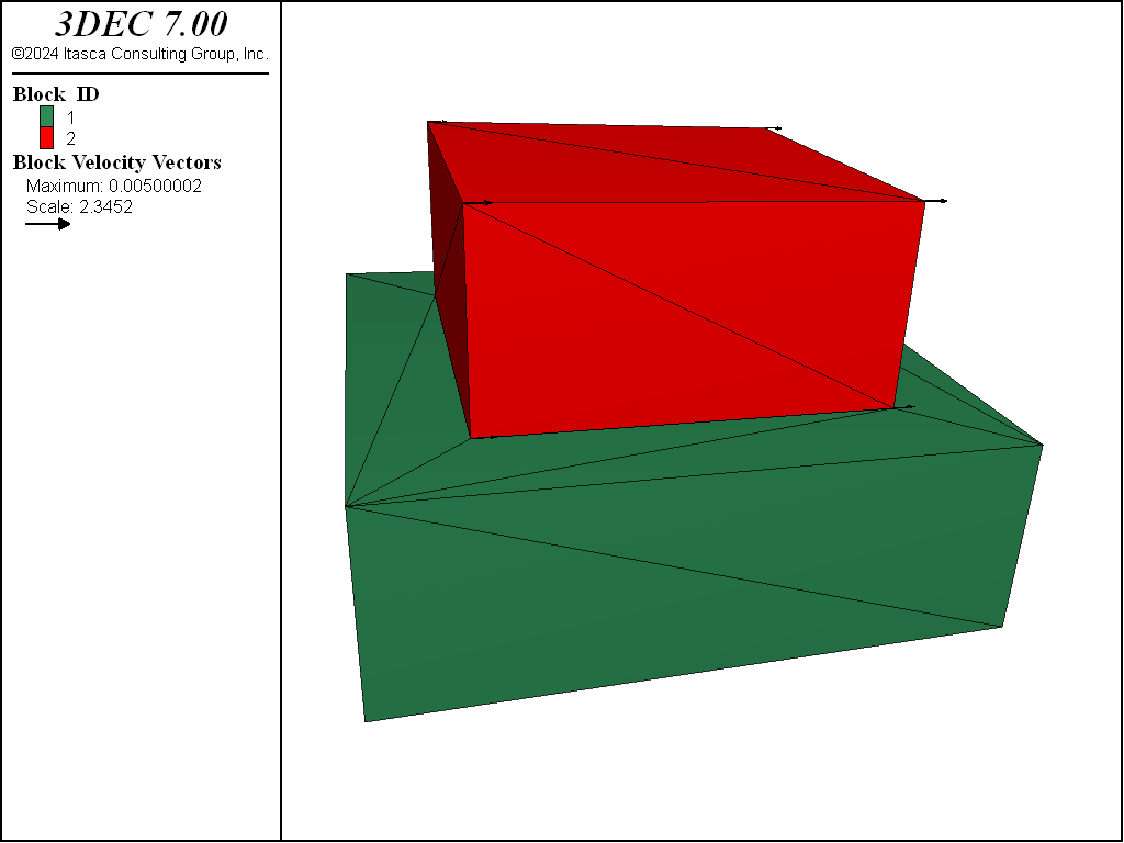
Figure 2: 3DEC model for direct shear test
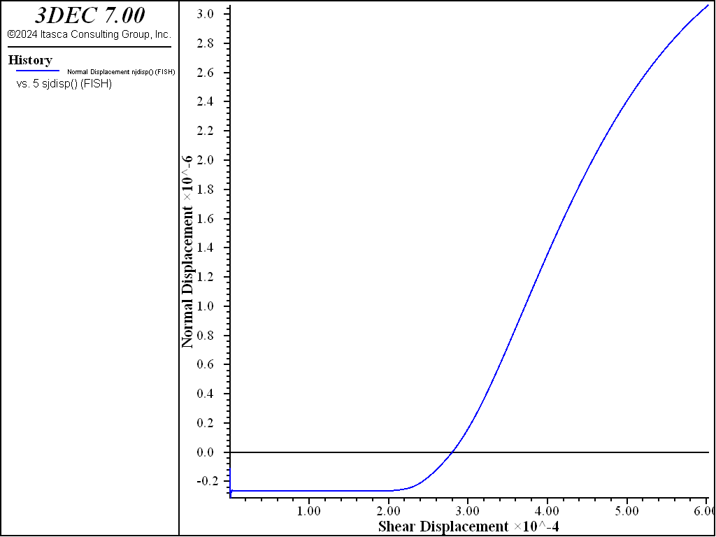
Figure 3(a) shows a plot of shear stress versus shear displacement for the case in which the joint initial friction is 59.3º. The normal displacement versus shear displacement plot for this assumption is shown in Figure 3(b). Similar plots of shear stress and normal displacement versus shear displacement for joint initial friction = 40.1º are given in Figure 4(a) and Figure 4(b).
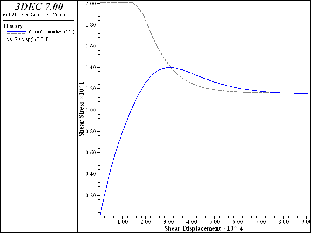
(a) shear stress (MPa) vs shear displacement (m).
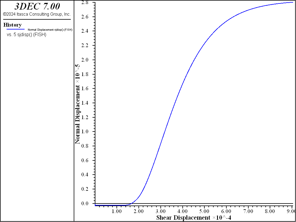
(b) normal displacement (m) vs shear displacement (m).
Figure 3: Results of direct shear test using continuously yielding model with initial joint friction at 59.3º.
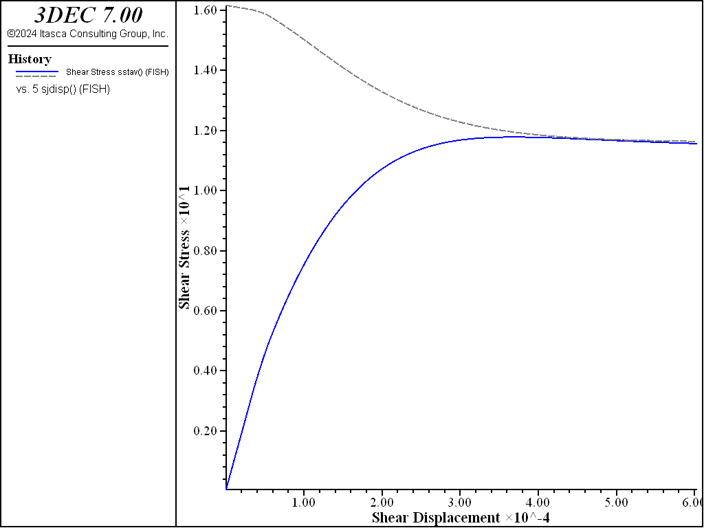
(a) shear stress (MPa) vs shear displacement (m).
(b) normal displacement (m) vs shear displacement (m).
Figure 4: Results of direct shear test using continuously yielding model with initial joint friction at 40.1º.
Data Files
cy_1.dat
model new
model large-strain off
;   file cy_1.dat
;   continuously yielding joint model
;   direct shear test
;   high peak stress
;
block create brick  -0.15,0.15  -0.15,0.15  -0.10,0.0
block zone gen  edge  1.0
block create brick  -0.10,0.10   -0.1,0.10   0.0,0.10
block zone gen  edge  0.2
;
block zone cmodel assign elastic
block zone prop  density =0.0026  bulk=4000   shear=3000
;
;  C-Y joint model
block contact jmodel assign cyjm
block contact prop kn-initial=100000  ks-initial=100000  friction-residual=30.0
block contact prop  exponent-normal=0.0     exponent-shear=0.0
block contact prop roughness=1.0e-4
block contact prop friction-initial=59.3
;
block hide range pos-z 0 .1
block gridpoint apply vel-x 0 vel-z 0 range pos-z -1 0.01
block hide off
;
; normal load
block face apply stress 0 0 -20  0 0 0 range pos-z 0.1
;
model step 100

; function to calculate average shear and normal stresses
program call 'sstav.fis'
;
block contact reset disp
block gridpoint ini disp 0 0 0

; shear load
block hide range pos-z  -.1 0
block gridpoint apply  vel-x=0.005 range pos-z -.1 1.1
block hide off
block gridpoint apply  vel-y=0.0   range pos-z -.1 1.1
;
his interval 5
model hist  mechanical unbal-max
fish hist name 'Shear Stress' sstav
fish hist name 'Normal Stress' nstav
fish hist name 'Normal Displacement'  njdisp
fish hist name 'Shear Displacement' sjdisp
fish hist name 'Bounding Shear Stress' tau_m
model cyc 15000

program return
cy_2.dat
model new
model large-strain off

;   file cy_2.dat
;   continuously yielding joint model
;   direct shear test
;   low peak stress
;
block create brick  -0.15,0.15  -0.15,0.15  -0.10,0.0
block zone gen  edge  1.0
block create brick  -0.10,0.10   -0.1,0.10   0.0,0.10
block zone gen  edge  0.2
;
block zone cmodel assign elastic
block zone prop  density =0.0026  bulk=4000   shear=3000
;
;  C-Y joint model
block contact jmodel assign cyjm
block contact prop kn-initial=100000 ks-initial=100000 friction-residual=30.0
block contact prop exponent-norm=0.0 exponent-shear=0.0
block contact prop roughness=1.0e-4
block contact prop friction-initial=40.1

;
block hide range pos-z 0 .1
block gridpoint apply vel-x 0 vel-z 0 range pos-z -1 0.01
block hide off
;
; normal load
block face apply stress 0 0 -20  0 0 0 range pos-z 0.1
;
model step 100

; function to calculate average shear and normal stresses
program call 'sstav.fis'
;
block contact reset disp
block gridpoint ini disp 0 0 0

; shear load
block hide range pos-z  -.1 0
block gridpoint apply  vel-x=0.005 range pos-z -.1 1.1
block hide off
block gridpoint apply  vel-y=0.0   range pos-z -.1 1.1
;
his interval 5
model hist  mechanical unbal-max
fish hist name 'Shear Stress' sstav
fish hist name 'Normal Stress' nstav
fish hist name 'Normal Displacement'  njdisp
fish hist name 'Shear Displacement' sjdisp
fish hist name 'Bounding Shear Stress' tau_m
model cyc 10000

program return
Properties
- continuously-yielding
- al f
Loading parameter (read only).
- exponent-normal f
Joint normal stiffness exponent (input).
- exponent-shear f
Joint shear stiffness exponent (input).
- friction-initial f
Joint initial friction angle in degrees (input).
- friction-residual f
Joint residual friction angle in degrees (input).
- kn-current f
Current joint normal stiffness (read only).
- kn-initial f
Joint initial normal stiffness (input).
- kn-maximum f
Joint maximum normal stiffness (input).
- kn-minimum f
Joint minimum normal stiffness (input).
- ks-current f
Current joint shear stiffness (read only).
- ks-initial f
Joint initial shear stiffness (input).
- ks-maximum f
Joint maximum shear stiffness (input).
- ks-minimum f
Joint minimum shear stiffness (input).
- plastic-strain f
Plastic shear strain (read only).
- roughness f
Joint roughness parameter (input).
- sdisp-peak f
Shear displacement magnitude at maximum shear stress (read only).
- sdisp-residual f
Shear displacement magnitude at start of residual shear stress (read only).
- sdisp f
Shear displacement magnitude at start of last discharge (read only).
- sstress-maximum f
Bounding shear stress (read only).
- sstress-peak f
Peak shear stress (read only).
- tol f
Tolerance to assess residual state. Default is 1e-5. (input).
- ussisref f
Shear displacement magnitude of reference (read only).
References
Cundall, P. A., and R. D. Hart. “Analysis of Block Test No. 1 Inelastic Rock Mass Behavior: Phase 2 – A Characterization of Joint Behavior (Final Report).” Itasca Consulting Group Report, Rockwell Hanford Operations, Subcontract SA-957 (1984).
Cundall, P. A., and J. V. Lemos. “Numerical Simulation of Fault Instabilities with a Continuously Yielding Joint Model,” in Rockbursts and Seismicity in Mines, pp. 147-152. C. Fairhurst, ed. Rotterdam: A. A. Balkema (1990).
Dafalias, Y. F., and L. R. Herrmann. “Bounding Surface Formulation of Soil Plasticity,” in Soil Mechanics – Transient and Cyclic Loads, Vol. 10, pp. 253-282. Chichester: John Wiley & Sons (1982).
| Was this helpful? ... | 3DEC © 2019, Itasca | Updated: Feb 25, 2024 |