Procedure for Dynamic Coupled Mechanical/Groundwater Simulations: Dam Foundation Wet
Note
To view this project in FLAC3D, use the menu command . Choose “Dynamic/DamFoundationWet” and select “DamFoundationWet.prj” to load. The main data files used are shown at the end of this example. The remaining data files can be found in the project.
The initial calculation stages for a coupled dynamic/groundwater analysis follow the same procedures as described for coupled static/groundwater analysis in Procedure for Dynamic Mechanical Simulations: Dam Foundation. The stages should lead to a mechanical equilibrium and steady groundwater flow state. The dynamic analysis is then performed following the four components.
The procedure for dynamic coupled simulations is illustrated by repeating the analysis of the earth dam in a steep valley. The grid generation stage (“GenGrid.dat”), the initial static equilibrium stage prior to reservoir loading (“GravLoad.dat”), and the application of the reservoir loading (“PropPlusWaterLoad.dat”) are identical in the coupled simulation.
The water from the reservoir is assumed to penetrate the dam this time, and a steady-state phreatic surface is calculated prior to earthquake loading. An uncoupled mechanical/groundwater analysis is performed first to determine the steady flow state and the final mechanical equilibrium state after filling of the reservoir. The dynamic analysis is then performed as a coupled simulation. The stages for this analysis are described below.
Initial Static Conditions with Phreatic Surface in Dam
This stage is begun after applying the reservoir loading to the dam, as described previously for “PropPlusWaterLoad.dat”. After applying the mechanical pressure to the upstream face of the dam, the dam deforms and the stress state readjusts as a result of the reservoir load. Note that this loading is imagined to take place rapidly, so that fluid flow is not allowed.
The fluid flow calculation mode is now turned on (model configure fluid). Only the final
flow pattern is of interest, not the time it takes to occur. (If consolidation time is
important, then consult Coupled Flow and Mechanical Calculations).
To allow rapid adjustment of the phreatic surface, begin from a fully saturated state
(zone gridpoint initialize saturation 1.0) and set the fluid modulus to a low
value (1 kPa, compared with the “real” value of 2 GPa for pure water). The fluid calculation and the mechanical adjustment are done separately because the fully coupled solution takes much longer (i.e., for this stage, model fluid active on and model mechanical active off). The tensile limit for water is set to zero so that a phreatic surface develops. Pore pressure is applied to the upstream face to correspond to the elevation of the reservoir. Pore pressure along the downstream face is fixed at zero to permit flow through this face, and pore pressure is set slightly above zero along the downstream toe to ensure that this surface will stay fully saturated. The data file for the flow-only stage is listed in “AddWater.dat”.
The pore pressure distribution at steady state is plotted in Figure 1. Gridpoint pore pressures are monitored during the flow calculation in the center of the dam and near the toe of the downstream slope. Histories of these pore pressures are plotted in Figure 2; these histories are a good indicator that steady state flow has been reached.
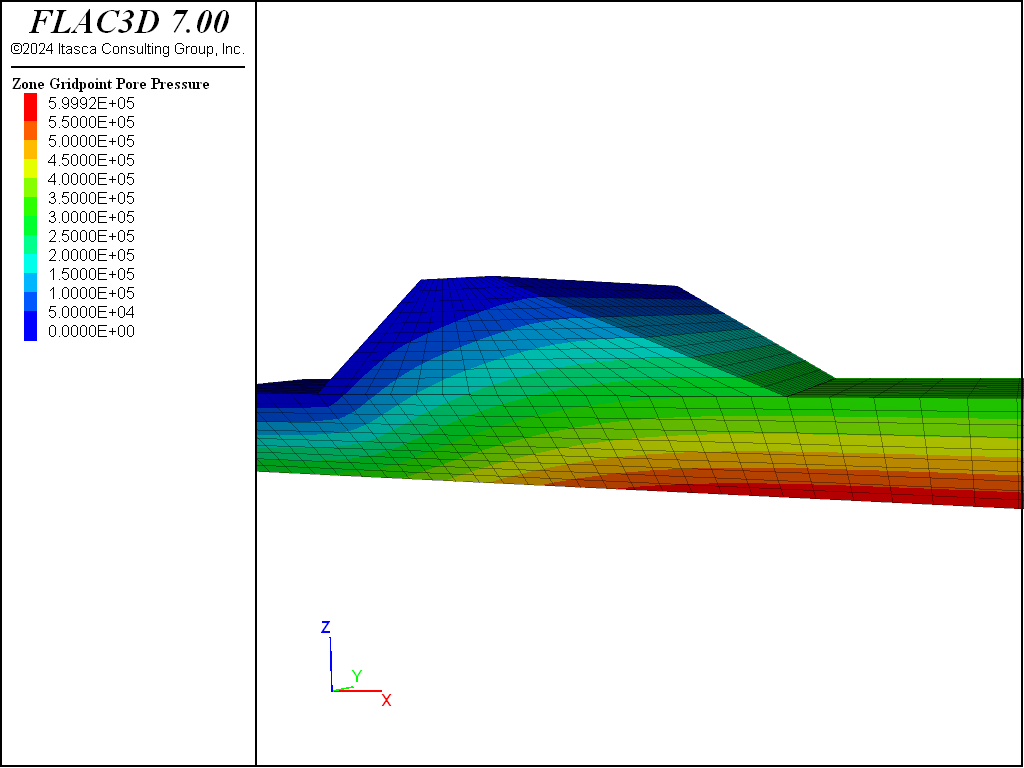
Figure 1: Pore pressure distribution after reservoir loading.
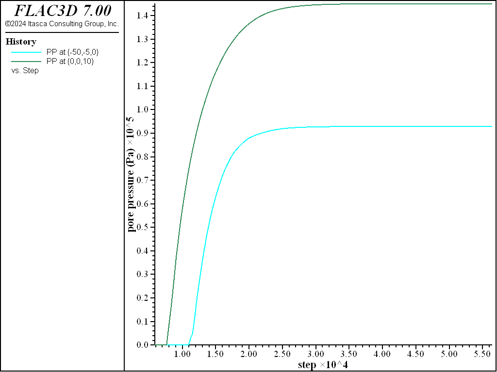
Figure 2: Pore pressure histories recorded at dam downstream toe (history 4) and at dam center (history 5).
Once the steady flow field is established, a final mechanical adjustment is needed because (a) some of the material is now partially saturated so the gravity loading is less, and (b) the effective stress state has changed, which may cause plastic flow to occur. During this stage, fluid flow and pore pressure changes are prevented (by setting fluid modulus temporarily to zero), because the consolidation process is not of concern here. See “MechAdjustWet.dat”.
Dynamic Analysis for Coupled Simulation
The dynamic simulation can now be performed. This is an undrained analysis; it is assumed that the duration of the earthquake loading is much shorter than the time for pore pressure dissipation resulting from groundwater flow. Pore pressure change in this case occurs only as a result of mechanical volume change resulting from the seismic shaking.
This modeling stage is essentially identical to that described in Dynamic Conditions and Simulation. The only difference is that a realistic value for the water bulk modulus is now included. A modulus of 0.2 GPa is selected, which is one order of magnitude smaller than the modulus of pure water. This value accounts for the presence of dissolved air within the soil. (See Fluid Bulk Modulus for further discussion.) The data file for the dynamic analysis stage is listed in “DynamicExcitationWet.dat”.
Additional deformation occurs in the dam during the dynamic loading as a result of the pore pressures within the dam. Figure 3 plots \(x\)- and \(z\)-displacement histories at the downstream edge of the dam crest, and Figure 4 shows the displacement contours and vectors at the end of the dynamic stage. The vertical settlement at the crest is approximately 200% more than that calculated in the previous case (compare Figure 3 to Figure 9). However, the deformation is more distributed through the downstream slope than before (compare Figure 4 to Figure 10).
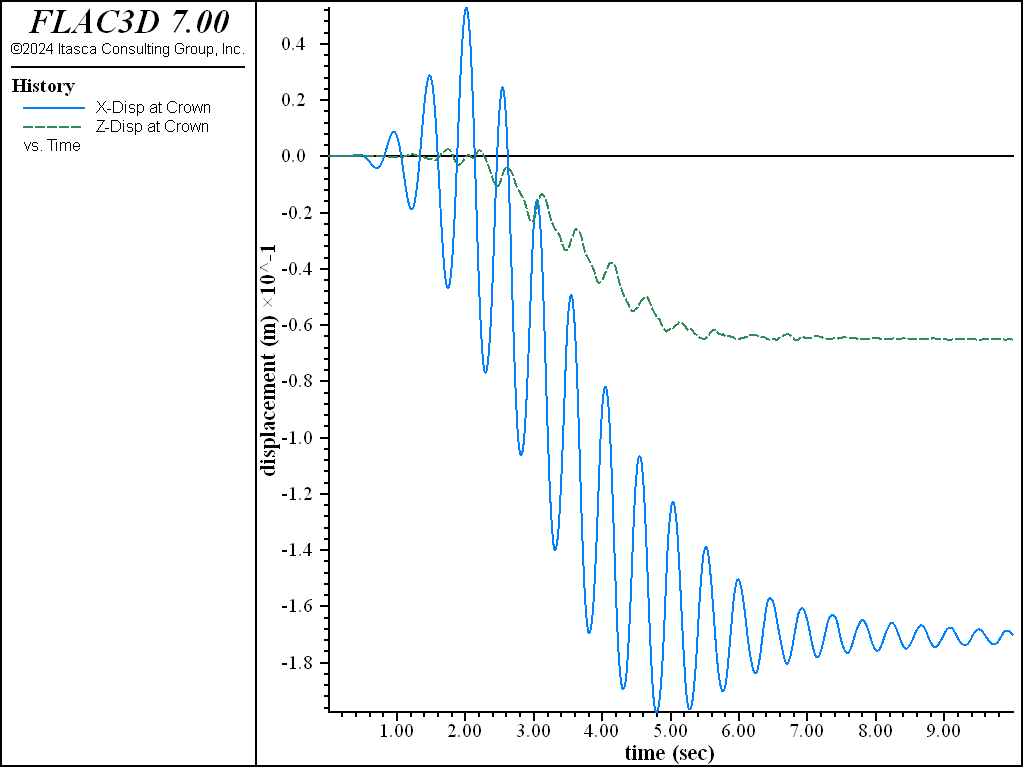
Figure 3: Displacement records (in x- and z-directions) at crest of dam — coupled response.
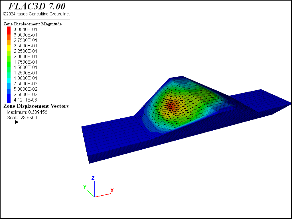
Figure 4: Contours and vectors of final displacement magnitude — coupled response.
No pore pressure build-up develops in this simulation because the Mohr-Coulomb model by itself does not include the effect of cyclic shear strain on volumetric strain. Some oscillation in pore pressure does occur during the dynamic loading, as shown by the pore pressure histories plotted in Figure 5.
Additional shear strain is also produced in this simulation, as can be seen by comparing the stress-strain plot in Figure 6 to that in Figure 11.
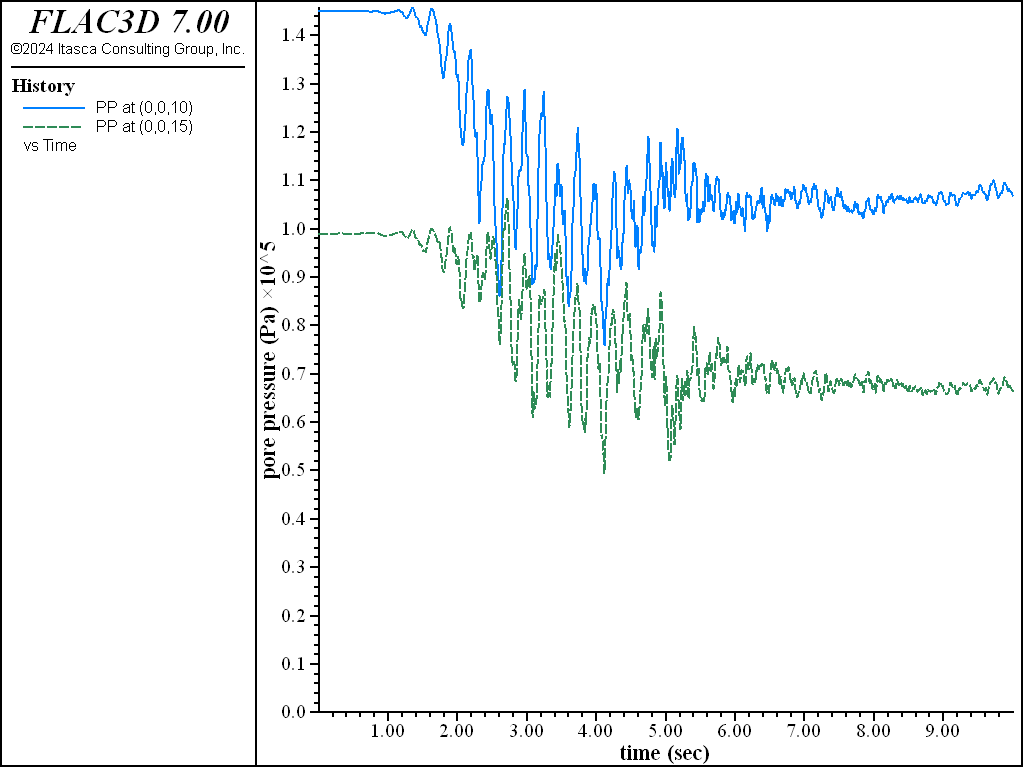
Figure 5: Pore pressure histories recorded at center of dam (history 28 at z=10, history 29 at z=15).
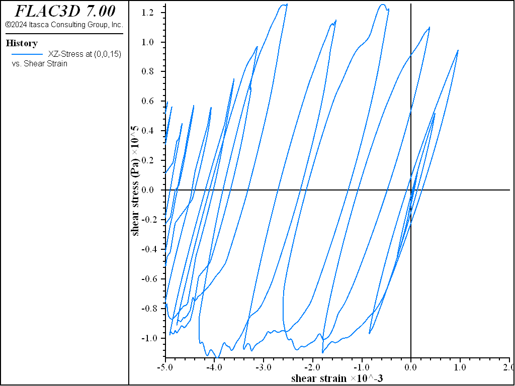
Figure 6: Shear stress versus shear strain at location (0,0,15) — Mohr-Coulomb material, hysteretic damped, coupled response.
Dynamic Pore-Pressure Generation
The dynamic coupled simulation is repeated with the Finn/Byrne constitutive model in order to simulate pore pressure generation and evaluate the potential for dynamic liquefaction. The dam is changed to liquefiable material by replacing the Mohr-Coulomb model with the Finn/Byrne model for the dam zones. Finn/Byrne parameters, \(C_1\) and \(C_2\), are specified assuming a normalized blow count of 15. Using this equation, \(C_1\) = 0.14736 and \(C_2\) = 1.35391. (See Simple Model Formulations.)
This simulation starts after the model is brought to mechanical equilibrium and steady-state fluid flow with the reservoir in place (i.e., after “MechAdjustWet.dat”). The dam zones are changed to Finn/Byrne material, and Finn/Byrne properties are assigned. Note that the stresses remain in the dam zones, even though the model is replaced. The model state is then checked with the new material to ensure that the system is still in equilibrium. The Finn/Byrne property, number-latency, is set to a large number (in this case, 100,000), and the model behaves the same as the Mohr-Coulomb model. number-latency is then set to 50 after equilibrium is checked so that shear-strain induced pore-pressure generation can occur during the cyclic dynamic loading. “FinnMaterial.dat” lists the commands for this stage.
The dynamic loading stage is now repeated by running “DynamicExcitationWet_finn.dat”. The same quantities as before are plotted. There is considerably more deformation in this case. The dam crest settles roughly 14 cm, and the downstream slope moves horizontally approximately 34 cm. Compare Figure 7 to Figure 3 and Figure 8 to Figure 4.
Pore pressure generation is now evident from the pore pressure histories plotted in Figure 9. Pore pressure builds up initially and then dissipates as the slope fails and deforms downstream.
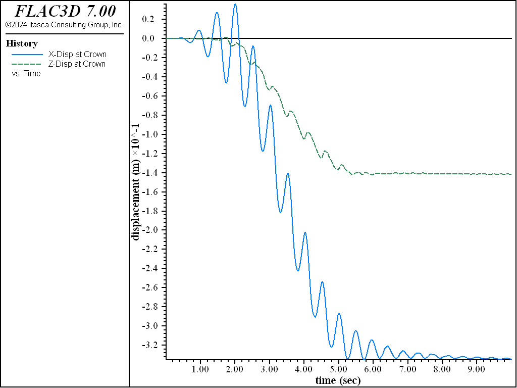
Figure 7: Displacement records (in x- and z-directions) at crest of dam — coupled response — Finn material.
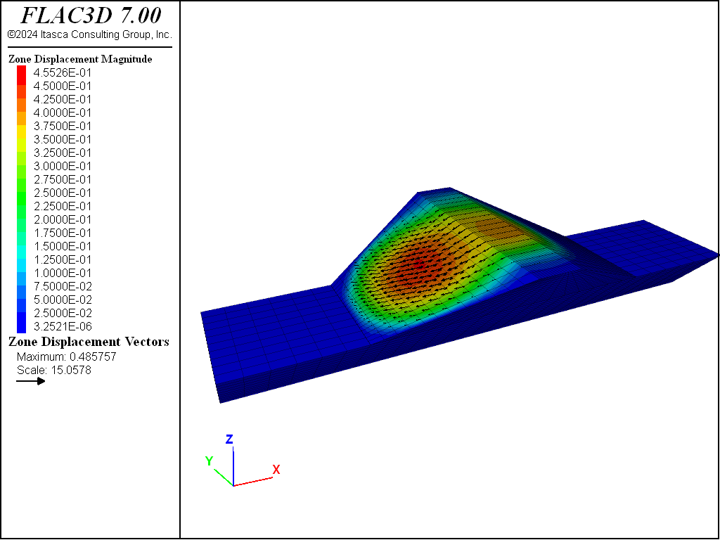
Figure 8: Contours and vectors of final displacement magnitude — coupled response — Finn material.
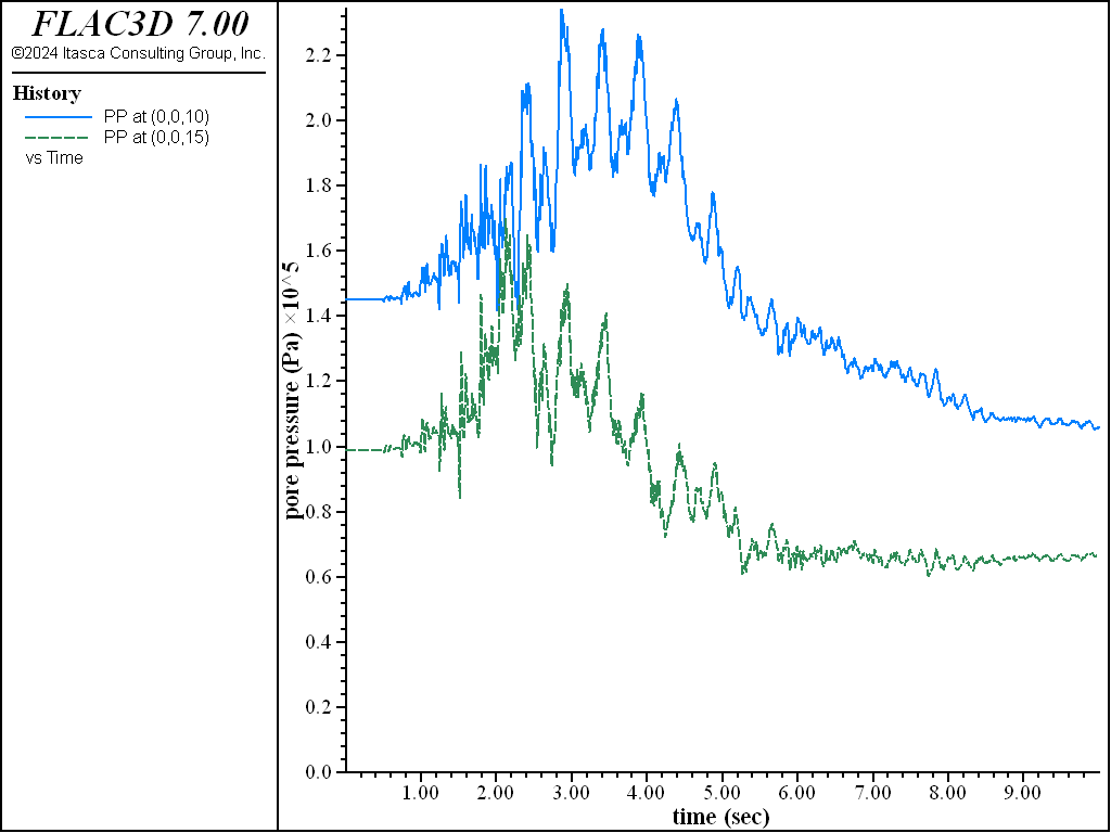
Figure 9: Pore pressure histories recorded at center of dam (history 24 at z = 10, history 26 at z = 15) — Finn material.
Data Files
Placement of foundation material - AddWater.dat
;------------------------------------------------------------
;       Dam and Foundation
;       Develop Phreatic Surface
;-------------------------------------------------------------------
model restore 'dam2'
model config fluid
zone fluid cmodel assign isotropic
model fluid on
model mech  off
zone gridpoint initialize fluid-modulus 1000.0
zone gridpoint initialize saturation 1.0
zone gridpoint initialize fluid-tension 0
zone fluid property porosity 0.3 permeability 1e-8
zone initialize fluid-density 1000
;
zone face apply pore-pressure=3e5 gradient (0,0,-1e4) ...
                                      range group 'Top2'
zone face apply pore-pressure=3e5     range group 'Top3' position-x 70 130
zone face apply pore-pressure=0.1     range group 'Top3' position-x -130 -70
zone face apply pore-pressure=0.0     range group 'Top1'
;
zone history name='pp1' pore-pressure position (-50,-5, 0)
zone history name='pp2' pore-pressure position (  0, 0,10)
;
model solve fluid ratio-flow 1.0e-5
model save 'dam2wet'
Mechanical adjustment to new flow field - MechAdjustWet.dat
;------------------------------------------------------------
;       Dam and Foundation
;       Mechanical adjustment after steady flow calculation
;-------------------------------------------------------------------
model restore 'dam2wet'
model fluid off
model mechanical on
zone gridpoint initialize fluid-modulus 0.0
model solve ratio-local 1e-4
model save 'dam2mechwet'
Assign Finn/Byrne material to dam - FinnMaterial.dat
;------------------------------------------------------------
;       Dam and Foundation
;       Change to Finn model
;-------------------------------------------------------------------
model restore 'dam2mechwet'
zone cmodel finn range group 'dam'
zone property shear 1e8 bulk 2e8 cohesion=40000 tension 4000  range group 'dam'
zone property friction 40 density 1700                        range group 'dam'
zone property constant-1 = 0.14736 constant-2 = 1.35391       range group 'dam'
zone property flag-switch = 1 number-latency = 1000000        range group 'dam'
model solve ratio-local 1e-4
zone property number-latency 50
model save 'dam2wetfinn'
Dynamic excitation of the dam/valley system — coupled analysis - DynamicExcitationWet.dat
;-----------------------------------------------------------------------
;       Dam and Foundation
;       Dynamic excitation of the dam/valley system - coupled simulation
;-----------------------------------------------------------------------
model restore 'dam2mechwet'
model dynamic active=on
model large-strain on
zone gridpoint initialize fluid-modulus 2e8
program call 'wave'
[table.as.list('vel') = table.integrate('acc')]
[table.as.list('dis') = table.integrate('vel')]
program call 'baseline' suppress
[baseline('vel',10,-0.00335,8,'cvel')]
[table.as.list('cdis') = table.integrate('cvel')]
; Apply quiet boundaries
zone face apply quiet range group 'East' or 'West'
; Apply corrected velocity history to base of model
zone face apply velocity (1,0.5,0) table 'cvel' ...
          range group 'North' or 'South' or 'Bottom2'
; Reset velocities and displacements
zone gridpoint initialize velocity (0,0,0)
zone gridpoint initialize displacement (0,0,0)
;
model history name='time' dynamic time-total
zone history name='xabase' acceleration-x position (0,0,-30)
zone history name='xacrest' acceleration-x position (0,0, 30)
zone history name='xdcrest' displacement-x position (-10,0,30)
zone history name='zdcrest' displacement-z position (-10,0,30)
zone history name='ssmid' strain-increment-xz position (0,0,15)
zone history name='sxzmid' stress-xz position (0,0,15)
zone history name='sstoe' strain-increment-xz position (-60,0,5)
zone history name='sxztoe' stress-xz position (-60,0,5)
zone history name='pp3' pore-pressure position (  0,0,10)
zone history name='pp4' pore-pressure position (  0,0,15)
zone history name='pp5' pore-pressure position (-50,0,10)
zone history name='pp6' pore-pressure position ( 50,0,10)
; Set damping values
zone dynamic damping hysteretic default -3.156 1.904
zone dynamic damping rayleigh 0.0005 2.0 stiffness
;
model solve time-total 10.0
model save 'dam3wetmc'
Dynamic excitation of the dam/valley system — coupled analysis - DynamicExcitationWet_finn.dat
;-----------------------------------------------------------------------
;       Dam and Foundation
;       Dynamic excitation of the dam/valley system - coupled simulation
;-----------------------------------------------------------------------
model restore 'dam2wetfinn'   ;  Finn model simulation'
model dynamic active=on
model large-strain on
zone gridpoint initialize fluid-modulus 2e8
program call 'wave'
[table.as.list('vel') = table.integrate('acc')]
[table.as.list('dis') = table.integrate('vel')]
program call 'baseline' suppress
[baseline('vel',10,-0.00335,8,'cvel')]
[table.as.list('cdis') = table.integrate('cvel')]
; Apply quiet boundaries
zone face apply quiet range group 'East' or 'West'
; Apply corrected velocity history to base of model
zone face apply velocity (1,0.5,0) table 'cvel' ...
          range group 'North' or 'South' or 'Bottom2'
; Reset velocities and displacements
zone gridpoint initialize velocity (0,0,0)
zone gridpoint initialize displacement (0,0,0)
;
model history name='time' dynamic time-total
zone history name='xabase' acceleration-x position (0,0,-30)
zone history name='xacrest' acceleration-x position (0,0, 30)
zone history name='xdcrest' displacement-x position (-10,0,30)
zone history name='zdcrest' displacement-z position (-10,0,30)
zone history name='ssmid' strain-increment-xz position (0,0,15)
zone history name='sxzmid' stress-xz position (0,0,15)
zone history name='sstoe' strain-increment-xz position (-60,0,5)
zone history name='sxztoe' stress-xz position (-60,0,5)
zone history name='pp3' pore-pressure position (  0,0,10)
zone history name='pp4' pore-pressure position (  0,0,15)
zone history name='pp5' pore-pressure position (-50,0,10)
zone history name='pp6' pore-pressure position ( 50,0,10)
;
zone dynamic damping hysteretic default -3.156 1.904
zone dynamic damping rayleigh 0.0005 2.0 stiffness
;
model solve time-total 10.0
model save 'dam3wetfinn'
⇐ Procedure for Dynamic Mechanical Simulations: Dam Foundation | Recommended Steps for Seismic Analyses ⇒
| Was this helpful? ... | FLAC3D © 2019, Itasca | Updated: Feb 25, 2024 |