Procedure for Dynamic Mechanical Simulations: Dam Foundation
Note
To view this project in FLAC3D, use the menu command . Choose “Dynamic/DamFoundation” and select “DamFoundation.prj” to load. The main data files used are shown at the end of this example. The remaining data files can be found in the project.
A simple model of an earth dam in a steep valley is used to illustrate most of the features used in a dynamic mechanical analysis. The dam is 30 m high, 60 m wide, and has a 20 m wide horizontal crest; the upstream and downstream slopes have grades of 2:1. It is assumed that the dam material can fail, and the riverbed foundation material does not fail as a result of the applied earthquake loading. The model is greatly simplified for the purposes of rapid execution, but it could easily be extended to represent a real dam (e.g., with a more complicated internal structure).
First, the stages leading up to the initial equilibrium state are described, followed by a description of the four components in the dynamic analysis, mentioned in Procedure for Dynamic Mechanical Simulations.
Grid Generation
The data file to set up the grid is given in “GenGrid.dat”. This in turn calls “Geometry.dat”, which was generated interactively using the Building Blocks pane and exported from the State Record pane. The resulting plot of the grid is shown in Figure 1. The dam, shown in green, rests on riverbed foundation material, shown in blue shading. Both are contained within boundary planes that represent a symmetrical valley with 45° slopes. For the purposes of this example, the valley material is assumed to be much stiffer than the dam and foundation materials, and is thus treated as a rigid boundary. It is represented by fixed boundaries rather than a separate grid.
The foundation material is simply truncated at both “ends” (boundaries in both
\(x\)-directions); in a more realistic model, these boundaries would be placed farther away.
Note that the grid is configured for a dynamic simulation at the beginning of the file
(model configure dynamic), but the dynamic mode of operation is “switched off” during
the initial, static stages (model dynamic active off).
The largest zone dimension in this grid is approximately 12 m. As discussed in Dynamic
Conditions and Simulation, this dimension is sufficient to
model wave propagation accurately in the model. The grid for the dam is made finer than that
for the riverbed foundation in order to provide a reasonable representation of any failure
region that may develop within the dam. The fine-grid dam is connected to the coarser-grid
foundation using the zone attach by-face command.

Figure 1: Grid for earth dam and foundation.
Initial Static Conditions
Boundary conditions are set up for the abutments and for the foundation ends such that motion is prevented normal to the corresponding planes when gravity is applied. In this way, the model reaches equilibrium with zero shear stresses on the boundary planes. The data file to achieve the initial equilibrium state is given in “GravLoad.dat”, and the resulting contour plot of vertical stresses is given in Figure 2. Note that the dam is composed of Mohr-Coulomb material, but its strength is set to prevent any yield during the initial compaction stage. Cohesion and tensile strength are set to large values. This approach to the installation of initial stresses is just one of many possible schemes; refer to Initial Conditions for a complete discussion of initial conditions.
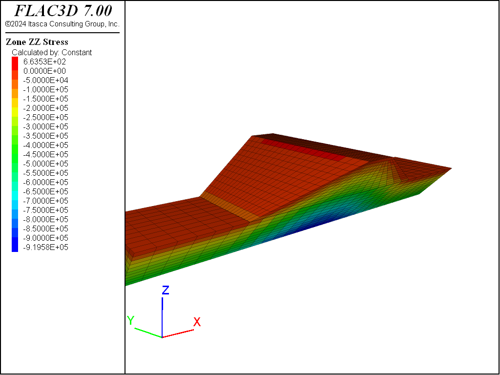
Figure 2: Contours of vertical stress after gravity loading.
The final stage in generating the initial static condition consists of setting realistic strength properties in the dam and applying pressure boundary conditions to the upstream side of the dam to simulate filling the reservoir. For the purposes of this illustrative example, the dam is assumed to be dry (i.e., the fluid simply acts as a mechanical boundary condition and does not penetrate the dam). In a more realistic analysis, a water table could be installed in the dam, leading to changed effective stresses in the dam. (This is demonstrated in the next section—see Dam Foundation Wet.) The material of the dam is assumed to have a cohesion of 40 kPa, a friction angle of 40°, and a tension limit of 4 kPa.
“PropPlusWaterLoad.dat” fixes all boundaries in the \(x\)-, \(y\)-, and \(z\)-directions (which implies a rough interface between the foundation materials and the rigid valley walls), sets the actual strength properties for the dam material, and applies a hydrostatic pressure to the upstream face of the dam to represent the reservoir loading. The foundation material remains elastic. The result of executing “PropPlusWaterLoad.dat” is that some yield occurs in the dam and the system stabilizes after a maximum displacement of roughly 1 cm along the upstream slope.
Dynamic Conditions and Simulation
The four components identified previously are now considered before performing the dynamic analysis.
Check Wave Transmission: The dynamic loading for this problem is a simplified motion: a sinusoidal acceleration wave applied at the base of the model in the horizontal direction. The wave has a frequency of 2 Hz and is applied in two components: one component is in the \(x\)-direction (along the valley) and has an amplitude of 2 m/sec2 (0.2 g); the other is in the \(y\)-direction (along the dam axis) and has an amplitude of 1 m/sec2 (0.1 g). An envelope function (\(\{1-\cos\omega t\}/2\)) 6 seconds in duration multiplies the 2 Hz input wave to provide a gradual build-up and decay of the wave. The acceleration equation for the wave, shown in Figure 3, is thus
(1)\[ \ddot u(t) = {1 \over 2} \ (1 - \cos({{\pi \over 3} t})) \ A \ \sin (2 \pi f t)\]where \(A\) is amplitude and \(f\) is frequency.
An acceleration record for a seismic analysis is typically read into the Dynamic Input Wizard and adjusted before being imported into FLAC3D. In this example, the record is created using a FISH function, wave, and store the record in a table (table ‘acc’) at a sampling interval of 0.002 seconds.
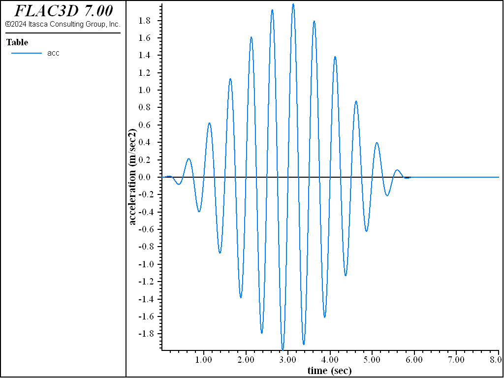
Figure 3: Input acceleration in x-direction (stored in table acc).
Based upon the elastic properties for this problem, the smaller compressional and shear wave speeds are in the dam and are (from P-Wave and S-Wave)
\(C_p\) = 443 m/sec
\(C_s\) = 243 m/sec
The largest zone dimension, \(\Delta l\), created for this model is 10 m. Based on frequency and element size, the maximum frequency that can be modeled accurately for propagating waves through the model is
(2)\[f = {{C_s} \over {\lambda}} = {{C_s} \over {10\ \Delta l}} \approx\ {\hbox { 2.4 Hz}}\]Therefore, the selected zone size is small enough to allow the waves at the input frequency of 2 Hz to propagate accurately.
Specify Damping: The plastic flow associated with the Mohr-Coulomb model dissipates considerable energy at high excitation levels. Hence, the selection of additional damping and damping parameters is less critical to the outcome of the analysis than if an elastic model were to be used throughout. Before applying any damping, check the maximum shear strains that can develop in the model, assuming elastic behavior, for the given dynamic loading conditions to evaluate if additional damping is appropriate.
If Rayleigh damping is used, a center frequency that reflects the frequencies associated with both the system and the input wave must be specified, as discussed in the Guidelines for Selecting Rayleigh Damping Parameters section. In this example, the input wave is of a single frequency of 2 Hz; hence, this value can be used as the Rayleigh center frequency. Alternatively, an undamped system could be excited by a single pulse; the resulting free oscillations would provide an estimate of the predominant natural periods of the system.
The other damping that can be use, “hysteretic” damping (as described in the Hysteretic Damping section), is independent of frequency. For this example, it is assumed that the dam and foundation materials behave as clayey soils with hysteretic behavior described by the modulus reduction curve shown here. If the default hysteretic damping function is used, described in Hysteretic Damping Formulation, with the values of \(L_1\) = -3.156 and \(L_2\) = 1.904, the hysteretic damping produces a reasonable fit to the modulus reduction and damping ratio curves up to a shear strain of approximately 0.1%, as shown in Comparison to SHAKE.
Note that a small amount of stiffness-proportional Rayleigh damping, usually less than 0.2%, can also be included with the hysteretic damping to remove any high frequency noise that may be observed in model results. (This is illustrated by the acceleration history plots in Figure 7 and Figure 8.)
Apply Dynamic Loading and Boundary Conditions: The
zone face applycommand is used with the table multiplier to specify the dynamic input. It is assumed that the acceleration, described by (2), is the motion that would occur at the valley sides, and thus a deconvolution of the wave is not necessary. The excitation can be applied by assuming either a rigid motion or compliant motion along the valley sides. In this example, it is assumed the excitation is applied as rigid motion along the sides. Alternatively, a flexible boundary may be simulated with the “quiet” option; a simple example using quiet boundaries is provided in Shear Wave Propagation in a Vertical Bar.The valley sides are fixed from movement in the \(z\)-direction. This implies a rough interface between the valley material and the riverbed foundation material. If differential movement between the valley material and riverbed material is anticipated, zones representing the valley material should be added and an interface installed between the materials.
The foundation material is terminated at 130 m from the dam crest line in both \(+x\) and \(-x\) directions. Quiet boundaries are prescribed at these ends to minimize reflection of secondary waves from the dam. Note that either condition (rigid or quiet boundary) causes a nonphysical effect on vertically propagating waves. (Free-field boundaries cannot be applied here because not all sides of the model are vertical.) Any artificial boundaries should be placed sufficiently far from the object of interest that their disruptive effects are minimized. Two or more simulations should be done with different boundary locations to determine the minimum distance for placement of the artificial boundaries such that their effects are negligible.
In general, it is easier to use the Dynamic Input Wizard (available from the Tools menu) to pre-process the input signal, including filtering and baseline correction. However, in this example, these steps are performed in FISH.
Before applying the input motion, the characteristics of the motion should be checked. The simple wave in this exercise has one dominant frequency: 2 Hz. However, in general, an input wave contains a range of frequencies. Filtering of a wave containing many frequency components may be necessary to remove high frequencies that can adversely affect wave propagation, as discussed in the Filtering section.
In addition, baseline drift should be checked (see Baseline Correction). In this exercise, the acceleration record (stored in table 1) is integrated twice using the FISH intrinsic
table.integrate. The velocity record is stored in table vel, and the displacement record in table dis. The resulting displacement record indicates a residual drift of -0.00335 m. Although this is considered to be insignificant and could be ignored, a correction is made for baseline drift to illustrate this procedure. A baseline correction is made by adding a low frequency sine wave (table 10) to the velocity record; the sine wave parameter is adjusted so that the final displacement will be zero. The corrected velocity is stored in table cvel, and the corrected displacement in table cdis. The correction routine is listed as “BASELINE.FIS” (see below).The uncorrected and corrected displacement records are shown in Figure 4.
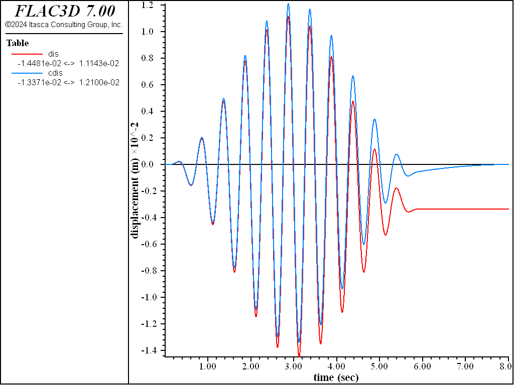
Figure 4: Uncorrected (table 3) and corrected (table 6) displacement histories.
The input motion is now applied using the baseline-corrected velocity record in table cvel. The command
zone face apply velocity(1,0.5,0) table cvel is used to apply \(x\)- and \(y\)-velocities with a range corresponding to the left and right valley sides, as shown in the data file “DynamicExcitation.dat”.Monitor Dynamic Response: In this example, velocities and accelerations are monitored in the \(x\)-direction at four depths under the dam crest, including the base (input wave). Displacement and stress components may also be monitored at any location. Cyclic shear stress versus shear strain plots are created to assess the maximum strain level and the amount of hysteretic deformational response that occurs in the materials. All histories should be requested before the dynamic simulation begins.
The data file for the dynamic simulation is “DynamicExcitation.dat”. Note that the solution mode is switched from static to dynamic mode (model dynamic active off) before the simulation begins, and a large-strain calculation is performed (model large-strain on). The FISH variables freq, ampl and env�_time denote the frequency of the input wave, the maximum amplitude of the wave, and the duration of the envelope, respectively.
The model is first run to check the elastic deformational response to dynamic loading, assuming undamped conditions. This helps evaluate whether additional damping is needed. Cyclic shear stress and shear strain histories are recorded at different locations in the model. In this case, the \(xz\) shear component of stress and strain is monitored. Figure 5 displays a shear stress versus shear strain plot in the center of the dam (0,0,15), and Figure 6 displays the same plot near the downstream slope at (-60,0,5) after a dynamic calculation period of 10 seconds. Peak shear strains are found to be less than 0.1% throughout the model. The default hysteretic damping, with parameters \(L_1\) = -3.156 and \(L_2\) = 1.904, is therefore considered to be appropriate to use for the dynamic loading range in this example.
Note that the stress/strain plots near the slope faces are not symmetric about the stress-strain origin, as indicated by Figure 6. This can cause an incompatibility between shear stress and strain when using hysteretic damping, as discussed in Practical Issues When Using Hysteretic Damping. In order to start from a compatible stress-strain state when dynamic loading is applied, it is more appropriate to initialize the static equilibrium state with hysteretic damping active. For this example, we assess that the incompatibility between shear stress and strain is confined to the slope faces, and that shear stresses are low through most of the model. Therefore, hysteretic damping is turned on after the model reaches static equilibrium. For a more thorough analysis, a simulation should also be made with hysteretic damping active from the start in order to assess the effect of the in-situ shear stresses.
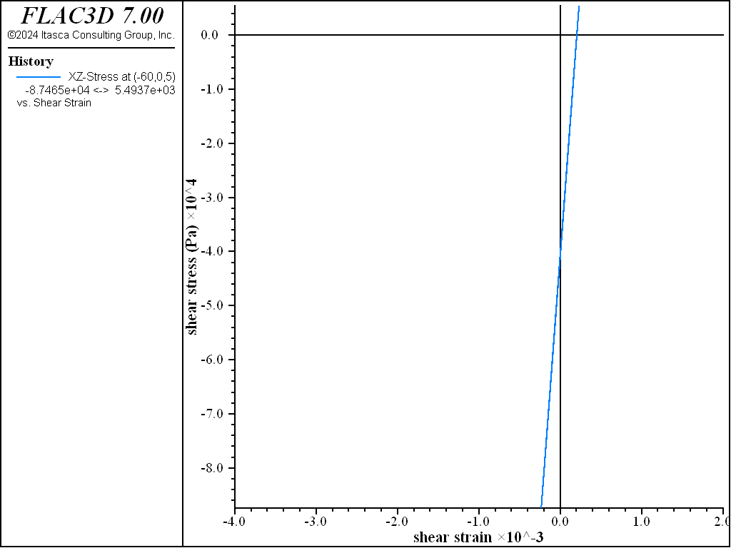
Figure 5: Shear stress versus shear strain at location (0,0,15) — elastic material, undamped.
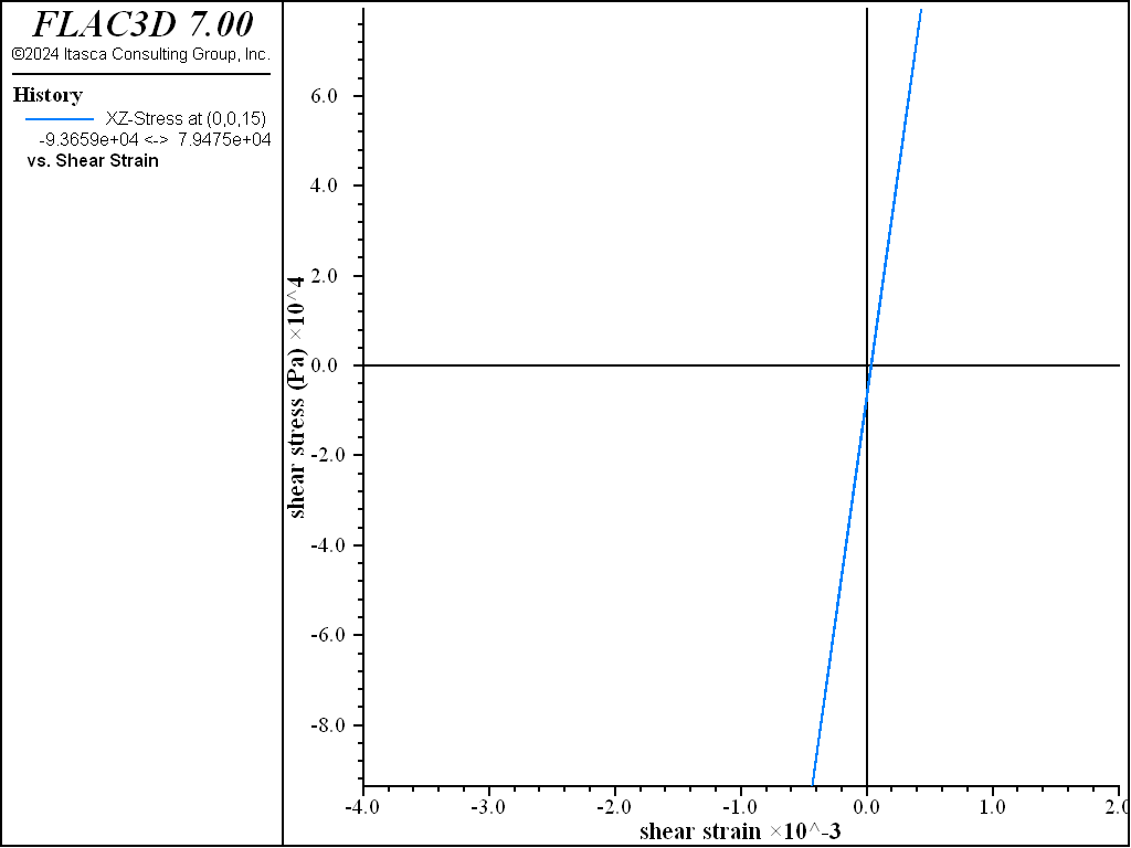
Figure 6: Shear stress versus shear strain at location (-60,0,5) — elastic material, undamped.
The model is now run with actual strength properties and the default hysteretic damping model. Figure 7 displays acceleration histories recorded at the model base and dam crest after a 10-second dynamic run. The \(x\)-acceleration response of the dam crest (dashed line) compared to the acceleration at the bottom of the model (solid line) is shown in the figure. There is an amplification factor of roughly eight; note that the crest accelerations are larger in the downstream (negative \(x\)-) direction.
Figure 7 shows high frequency noise in the acceleration toward the end of the simulation time. The dynamic stage is rerun with a small amount of stiffness-proportional Rayleigh damping (0.05% at 2 Hz) added to remove this noise. (See Figure 8.) This small amount of Rayleigh damping does not affect the deformations calculated in the model.
During the shaking, there is substantial plastic flow in the dam, which results in irrecoverable displacements. The \(x\)- and \(z\)-displacement histories at the downstream edge of the crest are shown in Figure 9; every cycle of oscillation causes an increment in displacement downstream and toward the abutment (due to the fact that the excitation is not aligned with the valley axis). A more comprehensive view of the final displacement field is shown in Figure 10 as contours and vectors superimposed on the dam surface. Slumping is observed concentrated near the crest on the downstream side.
The hysteretic response of the dam material is shown in Figure 11 and Figure 12. This response reflects the energy dissipated by both the plastic failure and the hysteretic damping.
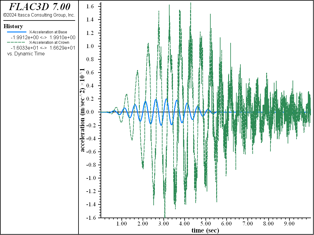
Figure 7: Acceleration histories for base (blue line) and crest (green line) — with only hysteretic damping
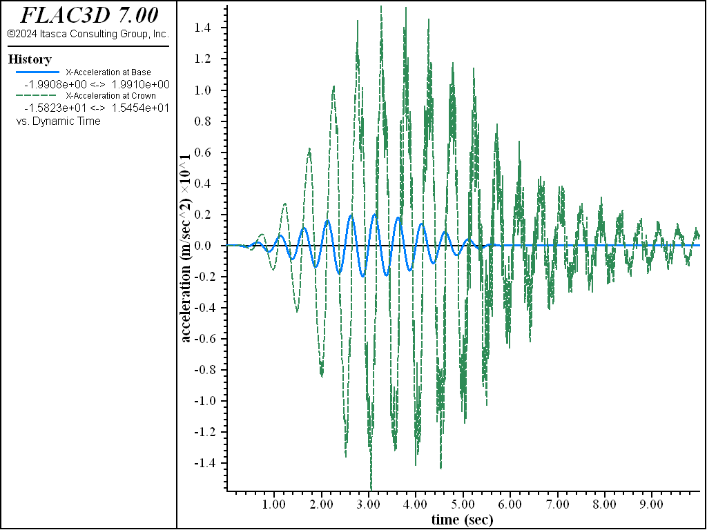
Figure 8: Acceleration histories for base (blue line) and crest (green line) — with hysteretic and 0.05% stiffness Rayleigh damping.
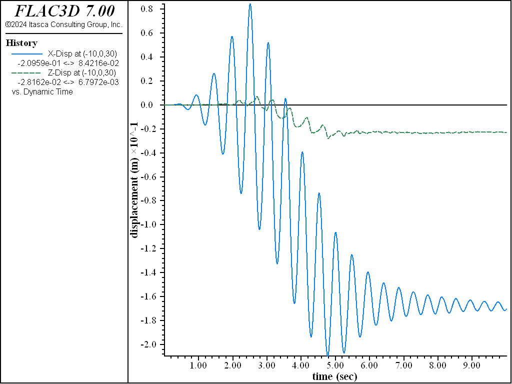
Figure 9: Displacement records (in x- and z-directions) at crest of dam.
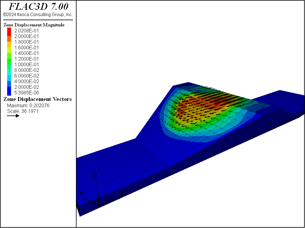
Figure 10: Contours and vectors of final displacement magnitude.
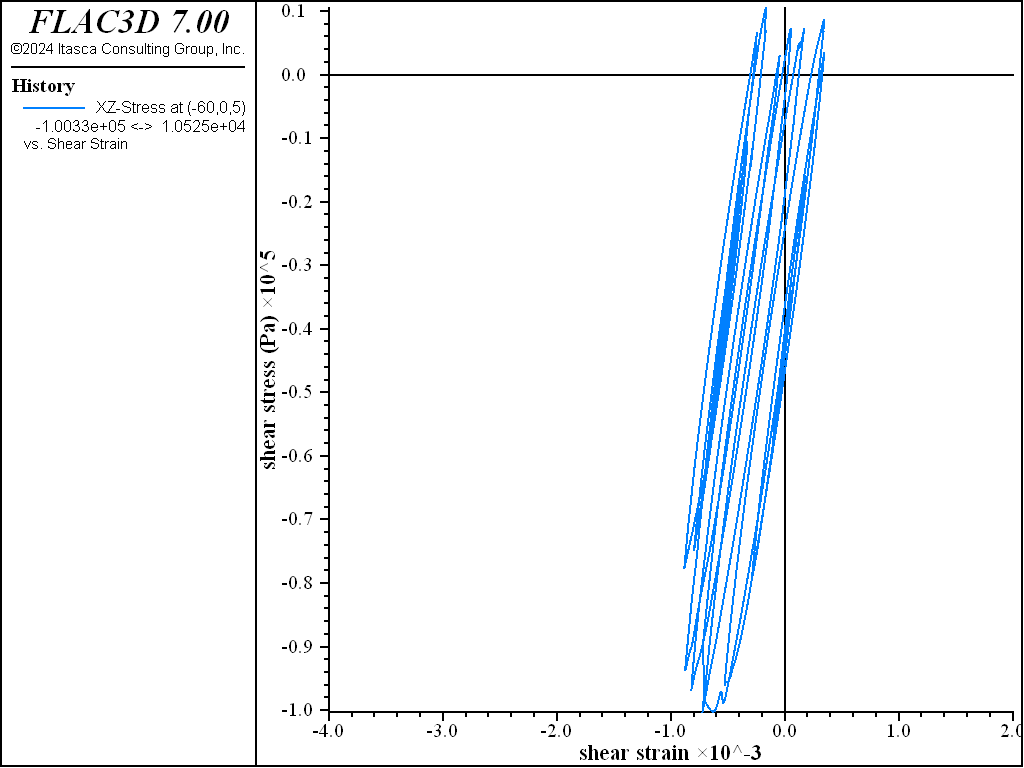
Figure 11: Shear stress versus shear strain at location (0,0,15) — Mohr-Coulomb material, hysteretic damped.
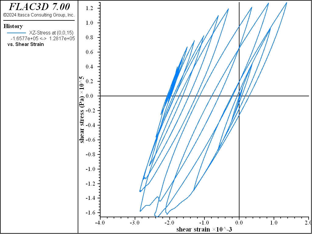
Figure 12: Shear stress versus shear strain at location (-60,0,5) — Mohr-Coulomb material, hysteretic damped.
Data Files
Generate grid for dam foundation - GenGrid.dat
;------------------------------------------------------------
;       Dam and Foundation
;       Generate grid
;-------------------------------------------------------------------
model new
model large-strain off
model config dynamic
model dynamic active off
;--- core ---
; generated geometry from GUI building blocks
program call 'Geometry' suppress
zone densify segments 1 2 1 range group 'dam'
; --- attach dam to foundation ---
zone attach by-face
; Assign constitutive model and properties
zone cmodel assign mohr-coulomb range group 'dam'
zone property shear 1e8 bulk 2e8 cohesion 1e10 tension 1e10 ...
              density 1700 range group 'dam'

zone cmodel assign elastic range group 'foundation'
zone property shear 5e8 bulk 1e9 density 2100  range group 'foundation'

model save 'dam0'
Apply boundary conditions and gravity loading - GravLoad.dat
;------------------------------------------------------------
;       Dam and Foundation
;       Apply gravity loading
;-------------------------------------------------------------------
model restore 'dam0'
; --- assign group names to boundaries
zone face skin break-angle 25
; --- apply zero normal velocity boundary conditions
zone face apply velocity-normal 0.0 range group 'North' or 'South'
zone face apply velocity-normal 0.0 range group 'East' or 'West'
model gravity 10
model solve convergence 1
model save 'dam1'
Set realistic strength properties and apply water load - PropPlusWaterLoad.dat
;------------------------------------------------------------
;       Dam and Foundation
;       Apply realistic properties and water load
;-------------------------------------------------------------------
model restore 'dam1'
zone gridpoint initialize displacement (0,0,0)
zone face apply-remove
zone face apply velocity (0,0,0) ...
          range group 'North' or 'South' or 'Bottom2' or 'East' or 'West'
zone face apply stress-normal -3e5 gradient (0,0,1e4) range group 'Top2'
zone initialize-stresses
zone property tension=4000 friction=40 cohesion=40000 range group 'dam'
model solve ratio-local 1e-4
model save 'dam2'
Dynamic excitation of the dam/valley system - DynamicExcitation.dat
;-------------------------------------------------------------------
;       Dam and Foundation
;       Dynamic excitation of the dam/valley system
;-------------------------------------------------------------------
model restore 'dam2'
model dynamic active=on
model large-strain on
; FISH function that calculated the applied wave, and stores it in table 'acc'
program call 'wave'
[table.as.list('vel') = table.integrate('acc')]
           ; Integrate acceleration to velocity
[table.as.list('dis') = table.integrate('vel')]
           ; Integrate acceleration to velocity
program call 'baseline' suppress
[baseline('vel',10,-0.00335,8,'cvel')] ; Baseline correct velocity
[table.as.list('cdis') = table.integrate('cvel')]
; Apply quiet boundaries
zone face apply quiet range group 'East' or 'West'
; Apply velocity to base
zone face apply velocity (1,0.5,0) table 'cvel' ...
                range group 'South' or 'Bottom2' or 'North'
; Reset velocities and displacements
zone gridpoint initialize velocity (0,0,0)
zone gridpoint initialize displacement (0,0,0)
; Histories
model history name='time' dynamic time-total
zone history name='xabase' acceleration-x position (0,0,-30)
zone history name='xacrest' acceleration-x position (0,0, 30)
zone history name='xdcrest' displacement-x position (-10,0,30)
zone history name='zdcrest' displacement-z position (-10,0,30)
zone history name='ssmid' strain-increment-xz position (0,0,15)
zone history name='sxzmid' stress-xz position (0,0,15)
zone history name='sstoe' strain-increment-xz position (-60,0,5)
zone history name='sxztoe' stress-xz position (-60,0,5)
; Specify damping, hysteretic and rayleigh
zone dynamic damping hysteretic default -3.156 1.904
zone dynamic damping rayleigh 0.0005 2.0 stiffness
; Solve to dynamic time 10
model solve time-total 10
model save 'dam3'
BASELINE.FIS
;Name:baseline
;Input:itab_unc/int/102/uncorrected velocity table
;Input:itab_corr/int/120/low frequency sine wave correction
;Input:drift/float/0.3/residual displ. at end of record
;Input:ttime/float/40.0/total time of record
;Input:itab_cvel/int/105/baseline corrected velocity
;Note:Perform baseline correction with low frequency sine wave
fish define baseline(itab_unc,itab_corr,drift,ttime,itab_cvel)
    local npnts = table.size(itab_unc)
    loop local ii (1,npnts)
        local tt = float(ii-1) * ttime / float(npnts)
        local vv = math.pi * tt / ttime
        local cor_d = drift * math.pi / (2.0 * ttime)
        table(itab_corr,tt) = -(cor_d*math.sin(vv))
        table(itab_cvel,table.x(itab_unc,ii)) = table.y(itab_corr,ii) ...
                                                + table.y(itab_unc,ii)
    endloop
end
⇐ Solving Dynamic Problems | Procedure for Dynamic Coupled Mechanical/Groundwater Simulations: Dam Foundation Wet ⇒
| Was this helpful? ... | FLAC3D © 2019, Itasca | Updated: Feb 25, 2024 |