Examples • Example Applications

Full-Scale Test Wall in Sand (FLAC2D)

Problem Statement

Note

This project reproduces Example 6 from FLAC 8.1. The project file for this example is available to be viewed/run in FLAC2D.[1] The project’s main data files are shown at the end of this example.

A test wall is constructed in well-graded sand and supported by shotcrete, tiebacks and “soil nails” (ASCE 1988). The “nails” consist of No. 10 grade-60 steel bars grouted into the soil mass. The tiebacks are anchored over a 24-foot length by pressure grouting and are pretensioned at a lockoff load of 186.0 kips. A cross-section through the test wall is shown in Figure 1.

Key features of this problem include:

• eight excavation stages;

• emplaced support components at each excavation stage;

• pretensioning the tiebacks to the specified lockoff load; and

• development of forces in support components as a result of soil deformation.

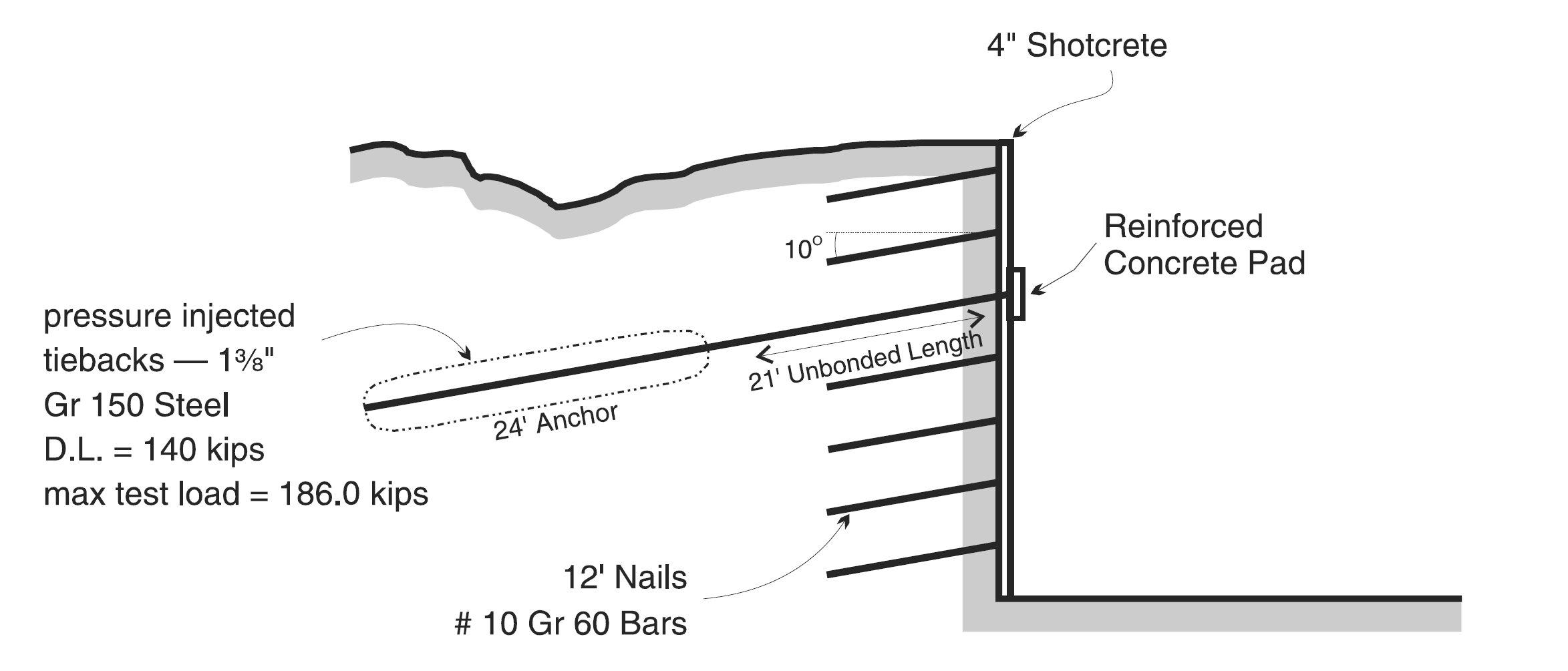
Figure 1: Cross-section through test wall.

The prototype wall consists of nails and tiebacks at regularly-spaced vertical and horizontal intervals. Reducing three-dimensional problems with regularly spaced reinforcement to two-dimensional problems involves averaging the reinforcement effect in three dimensions over the distance between the reinforcement. Donovan et al. (1984) suggest that linear scaling of material properties is a simple and convenient way of distributing the discrete effect of reinforcement over the distance between reinforcement in a regularly spaced pattern.

This approach is used in this analysis, based on a one-foot problem width and spacing for reinforcement as shown in Table 1. See Section xxx for a description of the properties that are scaled using this approach.

Table 1: Reinforcement spacing

Row	Spacing (feet)
1	4.5
2	3.5
3	9.0
4	4.5
5	4.5
6	4.5
7	4.5

Note that the spacing is the horizontal reinforcement spacing (in feet) for each of the seven rows for which the support components are installed.

The nails and tiebacks are assumed to be homogeneous, isotropic, linearly elastic materials represented as cables with the properties shown in Table 2.

Table 2: Properties for soil nails and tiebacks

Property	Row 1 Nails	Row 2 Nails	Row 3 Nails	Grouted Tieback	Ungrouted Portion	Row 4-7 Nails
Young’s Modulus (psf)	4.2×109	4.2×109	4.2×109	4.2×109	4.2×109	4.2×109
Area (ft^2)	8.5×10-3	8.5×10-3	8.5×10-3	0.0103	0.0103	8.5×10-3
Bond Stiffness (lb_f/ft/ft)	6.3×107	6.3×107	6.3×107	6.3×107	0	6.3×107
Bond Strength (lb_f/ft)	5000	5000	6000	9000	0	6000
Yield Strength (lb/ft)	73620	73620	73620	222750	222750	73620

The pressure dependency of the grout bond strength for the soil nails and tiebacks is neglected for this analysis. See Simulation of Pull-Tests for Fully Bonded Rock Reinforcement (FLAC2D) for an example that includes the pressure dependency of the bond strength.

The tiebacks are assumed to be installed and pretensioned to a lockoff load of 168.0 kips before further excavation is performed.

Note that the spacing keyword is used with the struct property command to assign the spacing in accordance with Table 1. By assigning spacing, the appropriate input properties in Table 2 will be automatically scaled, and the actual forces in the cable elements will be automatically calculated for output of results.

The shotcrete is assumed to be a homogeneous, isotropic, linearly elastic material represented as a liner with the following properties.

Table 3: Properties for the wall

Young’s modulus	4.8×108 psf
Poisson’s ratio	0.2
moment of inertia	3.0×10-3 ft4
area	0.333 ft2

In this example, beams are used instead of liner elements since we assume that the wall is perfectly connected to the soil (there is no sliding interface in between). When using beams to represent continuous support out of the plane, it is necessary to divide the modulus by \(1 - \nu^2\) so the beams are deforming in plane strain rather than plane stress (the default for beams). Therefore, in this model, a value of \(E = 5.0 \times 10^8\) is used.

The soil is assumed both to be homogeneous and to behave as a Mohr-Coulomb material with the following properties:

Table 4: Properties for the soil

Young’s modulus	2.0×106 psf
Poisson’s ratio	0.25
density	3.63 slugs/ft3
friction	36 degrees
cohesion	0
dilation	7.5 degrees

Modeling Procedure

The numerical analysis is performed by first compacting the soil mass under gravity to establish equilibrium of in-situ conditions and then sequentially excavating to various levels and introducing support elements.

Model Geometry

The model zones can be created in several different ways.

1. Export the virtual grid from Example 06 in FLAC 8.1. This will produce a data file that can be opened and called in FLAC2D. Calling the data file generates a Sketch set with the complete mesh and groups, and also automatically creates the zones. An example is included with the project called geometry.f2dat.

2. Import a dxf, then create edges and mesh, and then generate the zones. An example dxf is included with the project (edges.dxf).

3. Draw the geometry from scratch in the Sketch workspace.

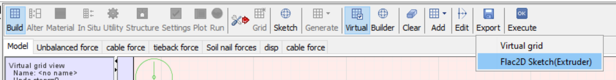
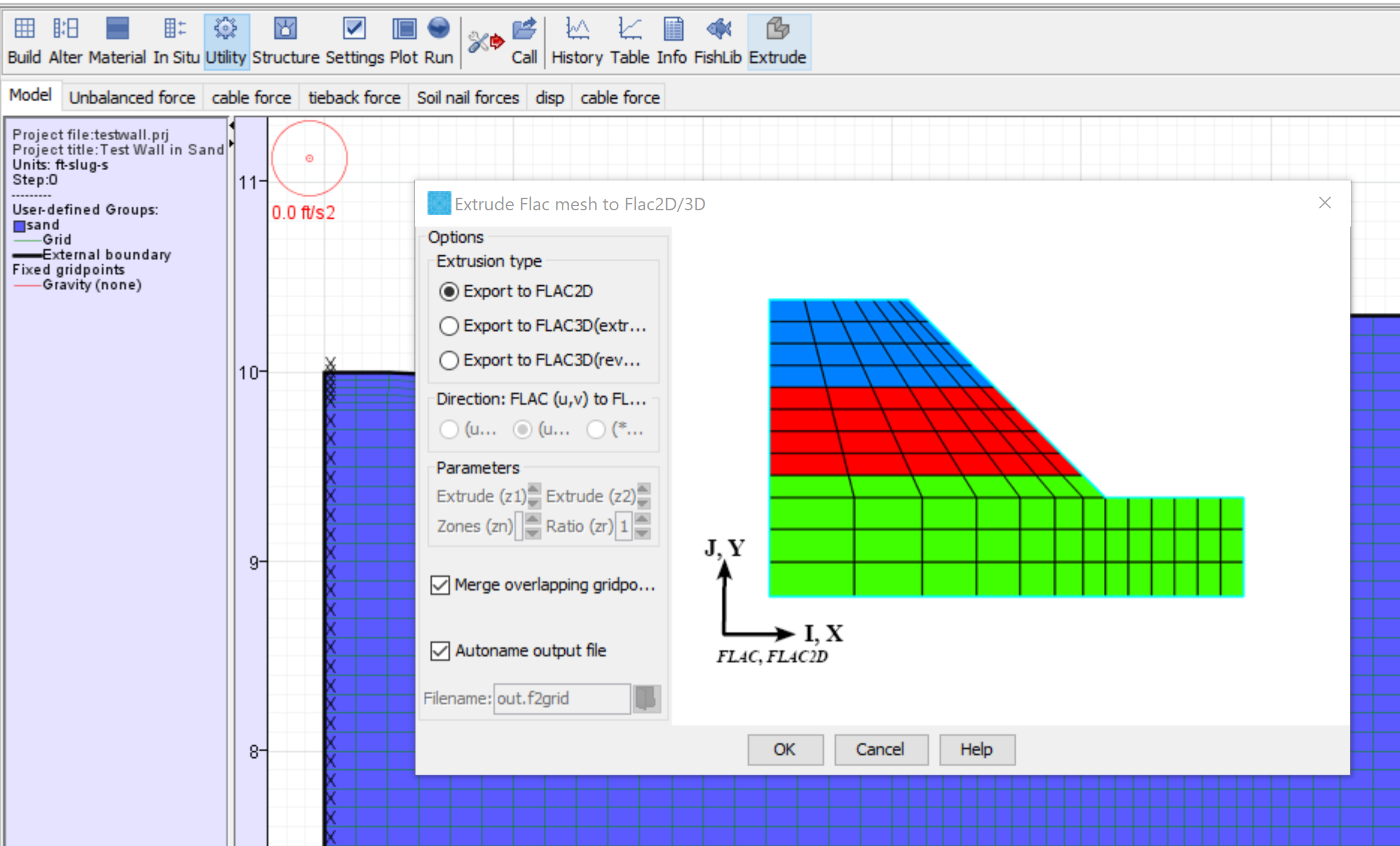
4. Export the FLAC 8.1 mesh to a grid file that can then be imported in FLAC2D with the zone import command. An example is included with the project called out.f2grd. This is less useful than importing or creating in the Sketch workspace because the different blocks that will be required to define the excavations are not delineated.

For this example, we will use method 2. Follow these steps to create the model geometry:

• Create a new Sketch set and import the file edges.dxf.

• Click the button on the toolbar to Automatically create edges from background geometry.

• Set the zone size for all Edges/Blocks to 1.5.

• Select all edges in the middle row of blocks (do this by first clicking on an edge, and then drawing a box around the middle section. This will highlight the selected edges as shown).

• Set the zone length for the selected edges to 1.

• All blocks could be meshed now, but this would result in an unstructured mesh, since there is a mismatch between the number of zones on the vertical edges. To obtain a structured mesh, do the following:

  • Select all of the vertical edges on the left and right side of the model.

  • Set the zone length to 1.

• Now, mesh all blocks.

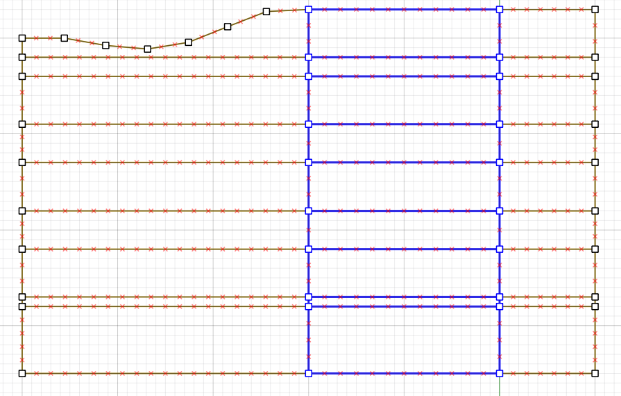
• Click the button to Create zones. The model should appear as in Figure 5.

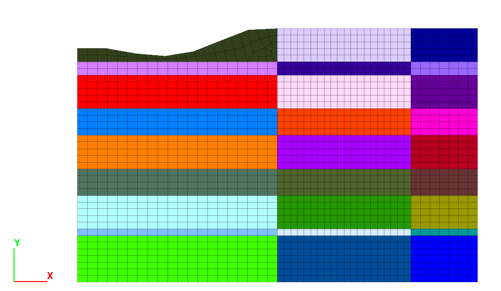
Figure 5: Final mesh

Note

The mesh in the top-left block is unstructured. This could be made a structured mesh by changing the top Points to Control Points. This is exemplified when importing the FLAC 8.1 virtual grid (see mesh generation method 1. above).

In the model pane, assign zone groups to the different stages of excavation as shown in Figure 6.

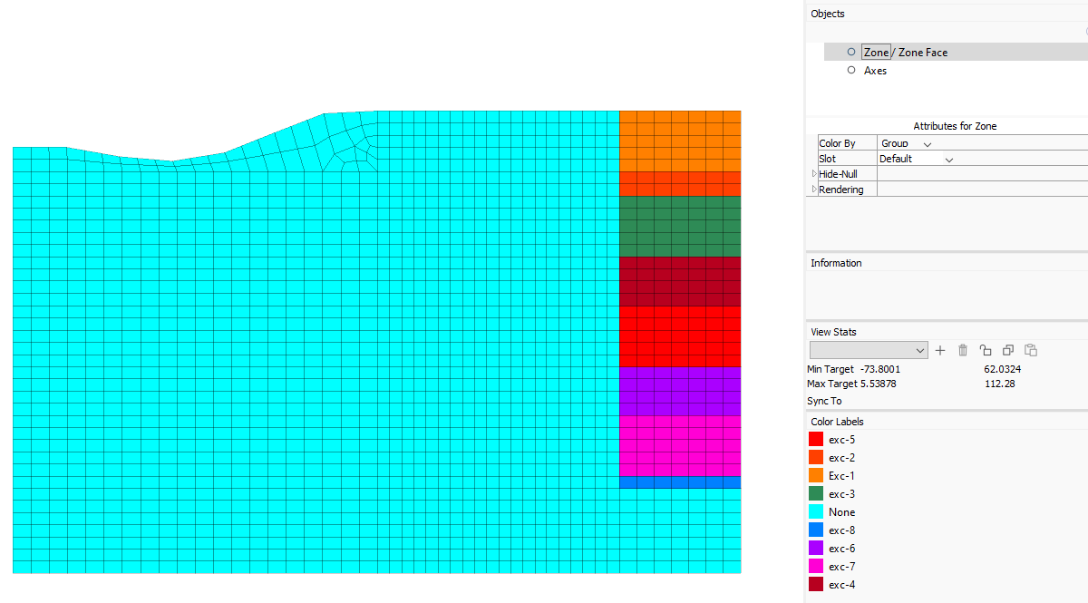
Figure 6: Zone groups

Now, press the button to Assign group names to faces automatically. Be sure to check the box to ignore existing group names.

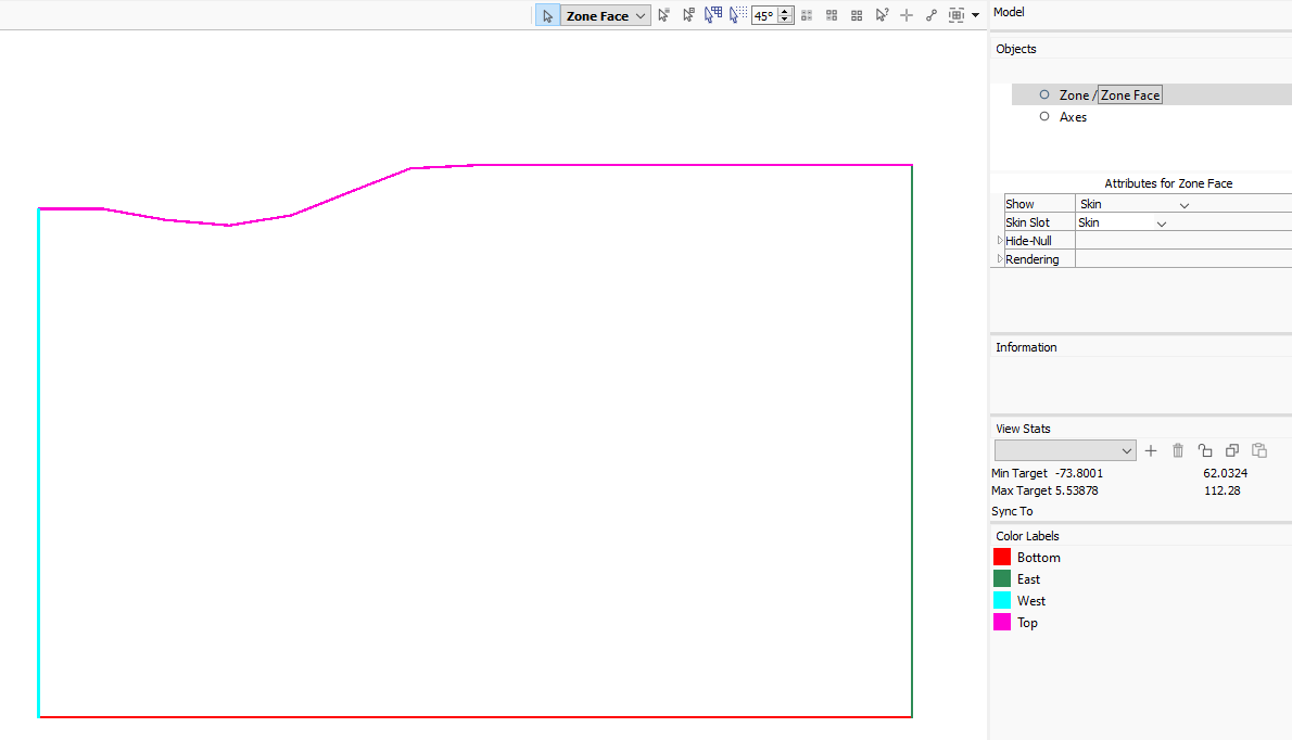
Figure 7: Automatically assigned face groups.

Now, assign face groups to the different segments of the wall. This will make it easier to attach structural elements later. To do this, follow these steps.

• Go back to plotting zones (rather than zone faces).

• Hide the group exc-1.

• Go back to the Zone Face Plot and under \(Show\), select Surface of Zones.

• Use the tool Select Faces along a polyline by break angle and then select the wall as shown.

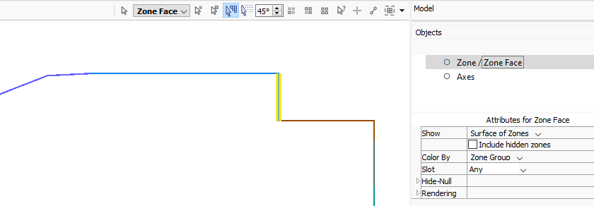
• Click Assign a group name to the selection, and name it wall-1.

• Go back to the Zone plot, show the previously hidden zones, and hide the zones for exc-2. Select the vertical wall segment and name it wall-2.

• Repeat for the next 6 wall segments.

The final plot of face groups should appear as in Figure 9.

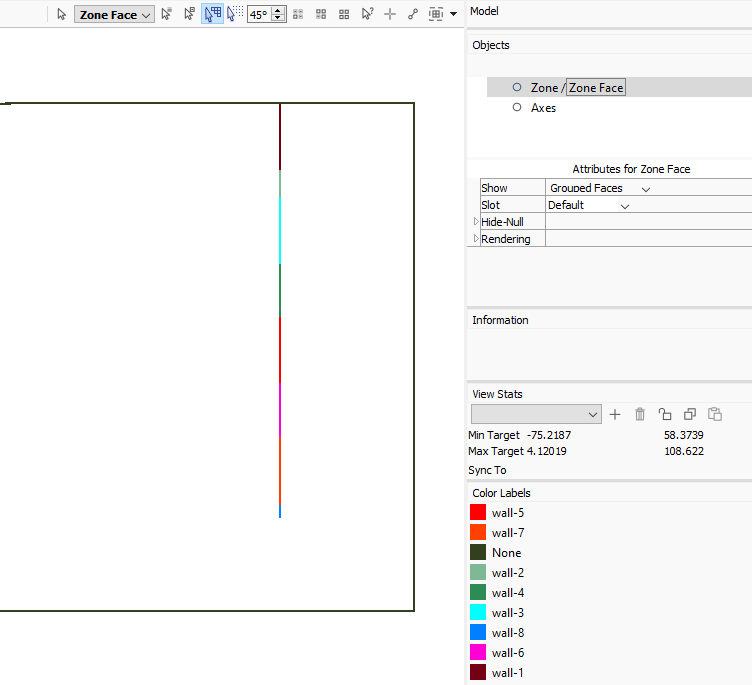
Figure 9: Face groups in the Default slot.

Finally, go back to the zone plot, show all zones, select all zones, and assign the Mohr-Coulomb constitutive model and properties as shown in Table 1.

Save the project and the model state.

Optional: Go to the State Record tab in the Commands area and save the record as a data file. This captures all the steps above as commands, which may be used later as needed in the project.

Initial Equilibrium

The data file used to set up boundary conditions, initial conditions and step to equilbrium is shown in initial.dat. Roller-boundary conditions are applied to the bottom and side boundaries. The ground surface is free (i.e., no applied stress). An initial stress state given by a coefficient of earth pressure at rest of 0.45 is assumed. The problem is then timestepped to equilibrium assuming large strain.

Excavation Stages 1 and 2

Note

When beam elements are created the same ID should be specified to ensure that they share nodes and the segments for each excavation stage are connected. If an ID is not given, it is assumed that the beam segments for each separate stage are not connected.

The first increment of excavation is modeled by deleting elements to a depth of 5 feet. At the same time, beam elements representing the shotcrete face support and cable elements representing the first row of soil nails are introduced. The model is stepped to equilibrium for this stage. This is then repeated for excavation stage 2.

Excavation Stage 3

The next increment is modeled by deleting zones equivalent to 5 feet of excavation. Shotcrete is installed as before. The tieback at this level is modeled using a ten-segment cable with a grouted unstressed length of 24 feet connected to a pretensioned one-segment cable with a length of 21 feet. A pretension force of 186.0 kips is applied to the ungrouted cable to simulate the effect of the pressure grouting. (Note that the pretensioning parameter is also scaled automatically by the tieback spacing of 9 feet.) The end of the tieback at the excavation face is connected directly to a gridpoint on the shotcrete in order to simulate the effect of the reinforced concrete pads.

Note that the snap keyword is used when making the tieback segments to ensure that the start node is at the same location as a node on the wall, and the start node of the grouted portion is at the same location as the end node of the ungrouted portion. Also note that the same ID is assigned to the two segments of the tieback to ensure that they share a node at the intersection point (the separate nodes could be joined instead with the command struct node join).

The pretensioning is performed by applying a tension force to the ungrouted portion, solving, and then removing the apply condition. The tension force will then be “locked in” to the ungrouted portion of the cable. The axial force after pretensioning is shown in Figure 10.

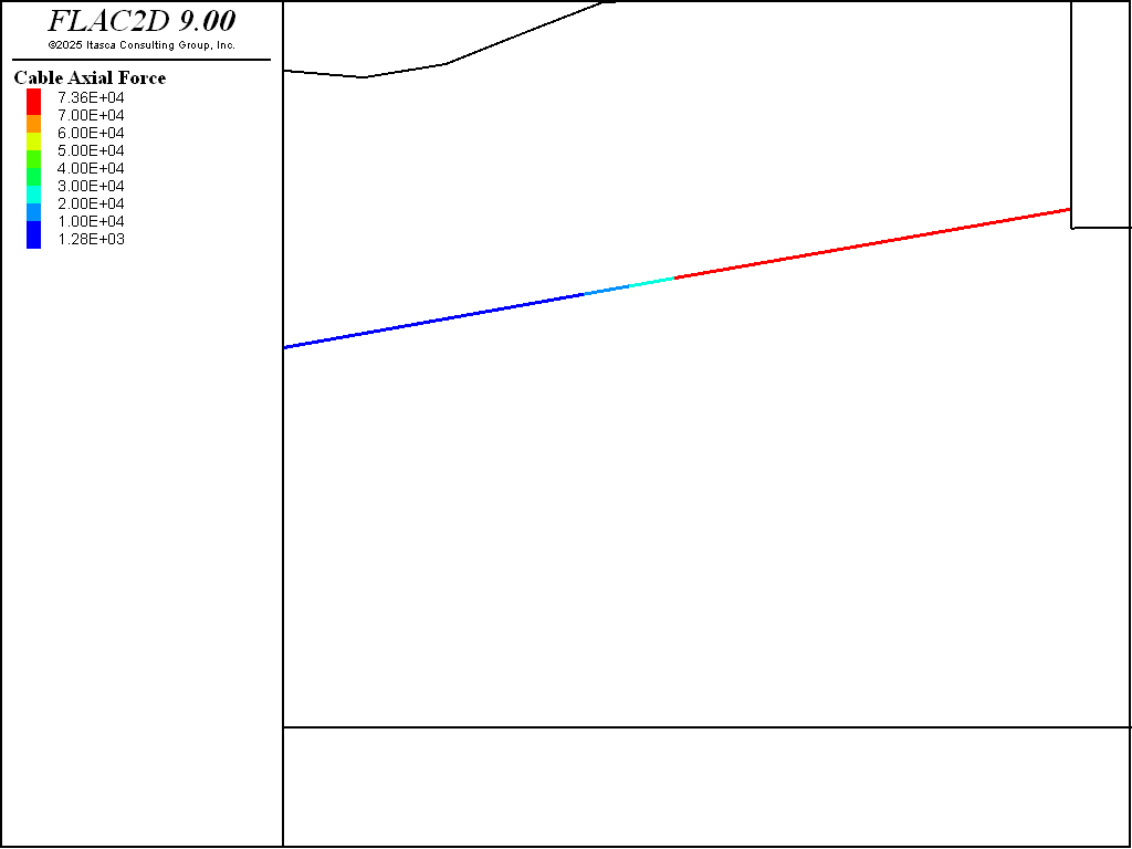
Figure 10: Axial forces in soil nails and tieback after the tieback is pretensioned.

Excavation Stages 4 - 7

The next four stages consist of deleting elements to simulate soil excavation, simultaneously installing support elements, and stepping to equilibrium to allow passive forces to develop in the reinforcement.

Excavation Stages 8

The final stage consists of deleting elements equivalent to one foot of excavation and simultaneously installing a liner element equivalent to one foot of shotcrete. The problem is then stepped to equilibrium.

The model at the completion of all excavation stages is shown in Figure 11.

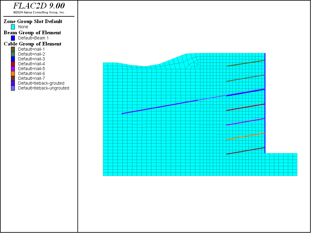
Figure 11: The model after all excavation stages.

Results

The results presented in Figure 12 through Figure 15 represent the state of the analysis following all excavation and support installation (i.e., the end of the analysis).

Figure 12 plots the actual axial forces in the soil nails and tiebacks at the last stage. Note that when spacing is specified with the struct prop command, the actual forces (and moments) are displayed in printed and plotted output for spaced structural elements.

Figure 13 and Figure 14 plot the actual forces along the tieback and soil nails, respectively, at the last stage. These plots are created using the FISH function tabforce contained in “make_tables.fis”. Scaled values for axial force are accessed directly in FLAC2D by the FISH function struct.cable.force.axial. These forces must be multiplied by the spacing to obtain the actual values, which are then stored in tables. The table numbers for the soil nail forces correspond to the excavation stages in which the nails were installed. Note that the peak value in the tieback force distribution plot in Figure 13 corresponds to the maximum axial force in the tieback (187 kips) (shown in Figure 12).

Figure 15 shows the displacements at the last stage and indicates the effect of the pretensioning in the tieback on reducing the movement of the wall. Intermediate results at the end of each stage, as well as displacement and loads in the shotcrete, are also available but are not presented here. Further discussion on this application is available in Lorig (1991).

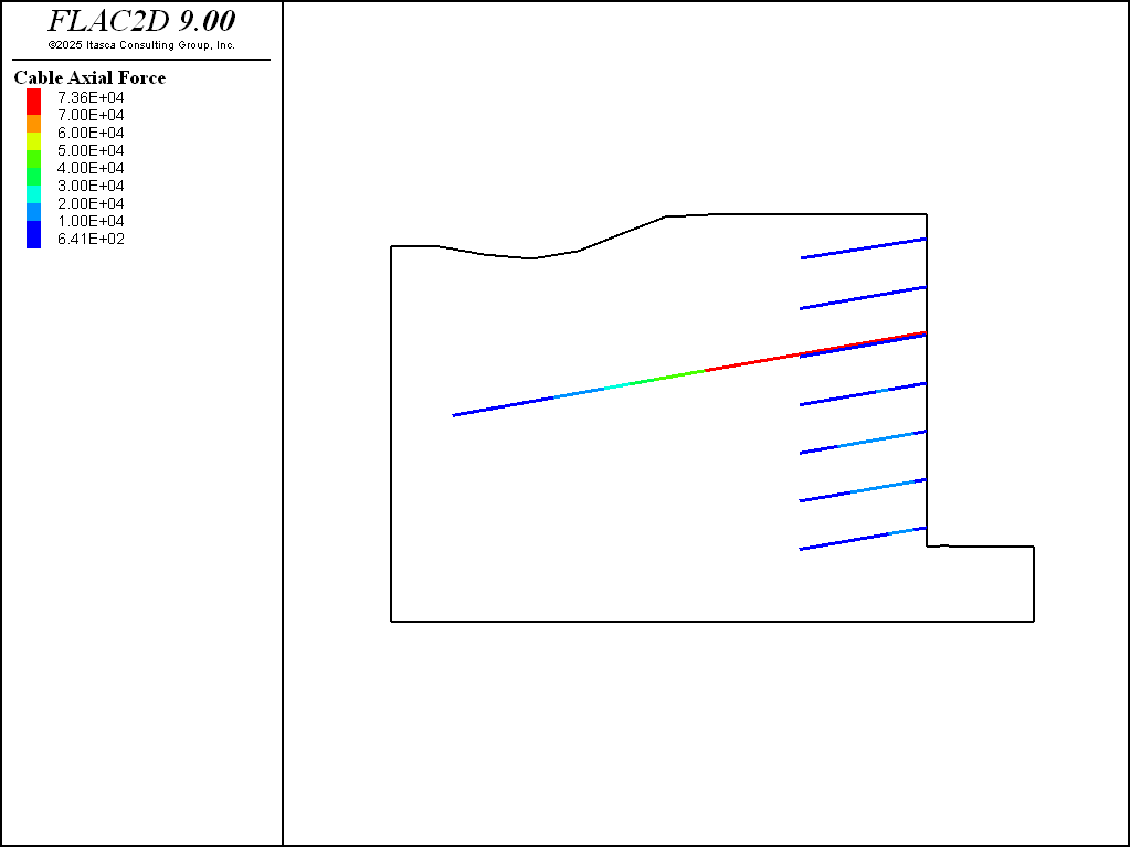
Figure 12: Actual axial tensile forces in the soil nails and tieback at the end of the analysis.

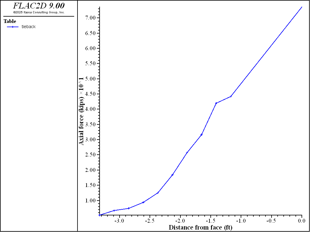
Figure 13: Distribution of axial tensile forces in the tieback.

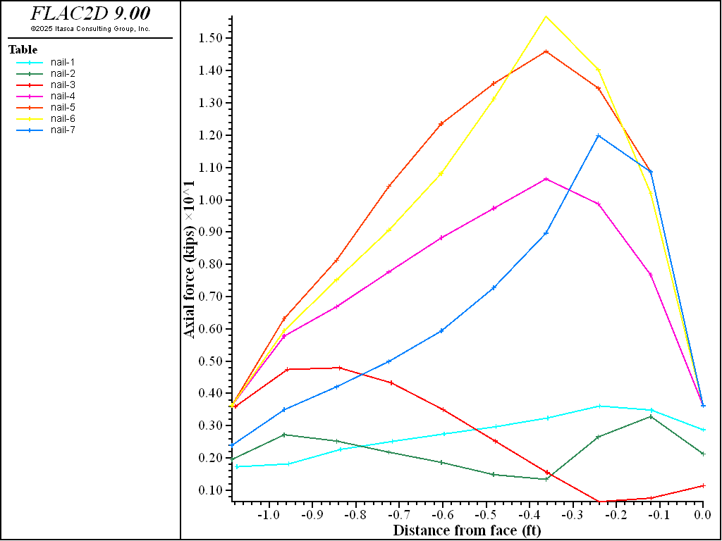
Figure 14: Distribution of axial tensile forces in the soil nails.

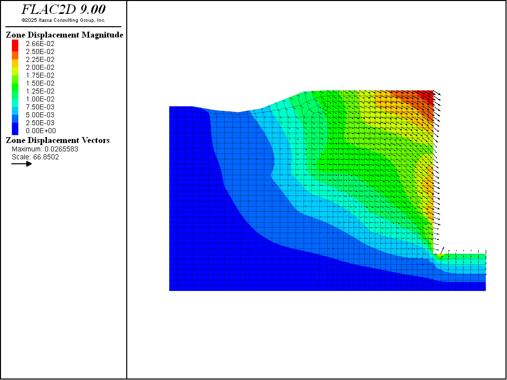
Figure 15: Displacement vectors for test wall analysis.

References

ASCE (American Society of Civil Engineers). “Full Scale Wall Tests Soil Nailing in Sand,” Civil Engineering, 58(5) (1988).

Donovan, K.,W. G. Pariseau and M. Cepak. “Finite Element Approach to Cable Bolting in Steeply Dipping VCR Stopes,” in Geomechanics Applications in Underground Hardrock Mining, pp. 65- 90. New York: AIME (1984).

Lorig, L. J. “Analysis of Novel Retaining Structures Using Explicit Finite Difference Codes,” in Computer Methods and Advances in Geomechanics, pp. 157-164. Rotterdam: A. A. Balkema (1991).

Data Files

initial.dat

model new

; model geometry, grouyps and properties from Sketch and Model pane
program call 'model'

; boundary conditions
zone face apply velocity-x 0 range group 'West' or 'East'
zone face apply velocity 0 0 range group 'Bottom'

; inital conditions
model gravity 32.185
zone initialize-stresses ratio 0.45

model large-strain on
model solve

model save 'initial'

excavation-1.dat

model restore 'initial'

; reset displacements to 0
zone gridpoint initialize displacement 0 0 

zone cmodel assign null range group 'exc-1'

; create wall
structure beam create by-zone-face id 1 range group 'wall-1'

; set properties.  Note that modulus is divided by 1-poiss^2 
; to account for continuity in the out-of-plane direction
structure beam property young=[4.8e8/(1.0-0.2^2)] poisson=0.20
structure beam property cross-sectional-area=0.333 moi=3.0e-3 

; add soil nail (cable)
; assign a group name since different cables will have different properties
; also set starting point slightly inside of zone to be safe
structure cable create by-line -0.01,100.75 -11.8,98.9 segments 10 group 'nail-1'
structure cable property cross-sectional-area=8.5e-3 young=4.2e9 ...
    yield-tension=73620 yield-compression 0 ...
    grout-stiffness=6.3e7 grout-cohesion=5000 spacing 4.5
                      
model solve
model save 'excavation-1'

excavation-3.dat

model restore 'excavation-2'

zone cmodel assign null range group 'exc-3'

structure beam create by-zone-face id 1 range group 'wall-3'

structure beam property young=[4.8e8/(1.0-0.2^2)] poisson=0.20
structure beam property cross-sectional-area=0.333 moi=3.0e-3

; install tieback before soil nail,
; otherwise tieback nodes will snap to soil nail nodes

; ungrouted section of tieback
; use SNAP to ensure first node is coincident with a node on the wall, also
; specify an ID number so the grouted and ungrouted sections will share a node
structure cable create by-line -0.001,92.0 -20.7,88.4 segments 1 ...
  group 'tieback-ungrouted' snap on ID 3

; grouted section of tieback -- use snap to ensure
; first node is at same location of last node of ungrouted section
structure cable create by-line -20.7,88.4 -44.3 84.2 segments 10 ...
  group 'tieback-grouted' snap ID 3

structure cable property cross-sectional-area=0.0103 young=4.2e9 ...
  yield-tension=73620 grout-stiffness=6.3e7 grout-cohesion=9000 spacing 9 ...
  range group 'tieback-grouted' or 'tieback-ungrouted'

; set cohesion to 0 for ungrouted portion
structure cable property grout-stiffness=0 range group 'tieback-ungrouted'

; join cable to wall
structure node join range group 'tieback-ungrouted'

; apply pretension to ungrouted part
structure cable apply tension value 186000 range group 'tieback-ungrouted'
model solve
structure cable apply tension active off

; soil nail
structure cable create by-line -0.1,91.75 -11.9,89.7 segments 10 group 'nail-3'
structure cable property cross-sectional-area=8.5e-3 young=4.2e9 ...
    yield-tension=73620  yield-compression 0 ...
    grout-stiffness=6.3e7 grout-cohesion=6000 spacing 9 ...
    range group 'nail-3'

; now solve
model solve
model save 'excavation-3'

make_tables.fis

; make tables plot graphs of force along cables
fish define make_tables

  ; make tables for soil nails
  table_pointers = list
  loop i (1,7)
    cable_group = 'nail-'+string(i)
    table.create(cable_group)
  end_loop
  
  ; make table for tieback
  table.create('tieback')
  
  ; get coordinates of element closest to wall (max x)
  ; and store in a list
  start_point = list(8)
  loop i (1,8)
    cable_group = 'nail-'+string(i)
    if i = 8
      cable_group = 'tieback-ungrouted'
    endif
    max_x = -1e20
    loop foreach el struct.list      
      if struct.group(el) = cable_group
        if struct.pos.x(el) > max_x
          max_x = struct.pos.x(el)
          start_point(i) = struct.pos(el)
        end_if
      endif
    end_loop
  end_loop
  
  ; now loop through elements and add values to tables
  loop foreach el struct.list
    ; soil nails
    loop i (1,7)
      cable_group = 'nail-'+string(i)
      distance = math.mag(struct.pos(el) - start_point(i))
      if struct.group(el) = cable_group
        ; make distance negative so the plot mimics the model
        ; make force in kips
        value = vector(-distance,struct.cable.force.axial(el)*0.001)
        command
          table [cable_group] insert [value]
        end_command
      endif
    end_loop
    
    ; tieback
    i = 8
    cable_group = 'tieback-ungrouted'
    distance = math.mag(struct.pos(el) - start_point(i))
    if struct.group(el) = cable_group
      value = vector(-distance,struct.cable.force.axial(el)*0.001)
      command
        table 'tieback' insert [value]
      end_command
    endif
    
    cable_group = 'tieback-grouted'
    distance = math.mag(struct.pos(el) - start_point(i))
    if struct.group(el) = cable_group
      value = vector(-distance,struct.cable.force.axial(el)*0.001)
      command
        table 'tieback' insert [value]
      end_command
    endif
  end_loop
end
[make_tables]
    
  

Endnotes

[1]

To view this project in FLAC2D, use the program menu.

Help ▼ Examples…

  ⮡   FLAC
   ⮡   Example Applications
    ⮡   FromFLAC
     ⮡   06TestWall
     ⮡   TestWall.prj