Examples • Example Applications

Wharf Subjected to Earthquake Loading (FLAC2D)

Problem Statement

Note

The project file for this example is available to be viewed/run in FLAC2D.[1] The project’s main data files are shown at the end of this example.

This is an illustrative example of a wharf subjected to earthquake loading. The model can be run in demonstration mode without a license. The soil profile, consisting of three layers (4.5 m, 6.5 m, and 11.0 m), is shown in Figure 1. The water table is 2 m below the sloping ground. The slope contains sand that may spread laterally during an earthquake. This spreading could push the piles and potentially compromise the safety of the wharf. However, the piles also have a spinning effect that can reduce the lateral spreading of the slope. This is an example of soil-structure interaction.

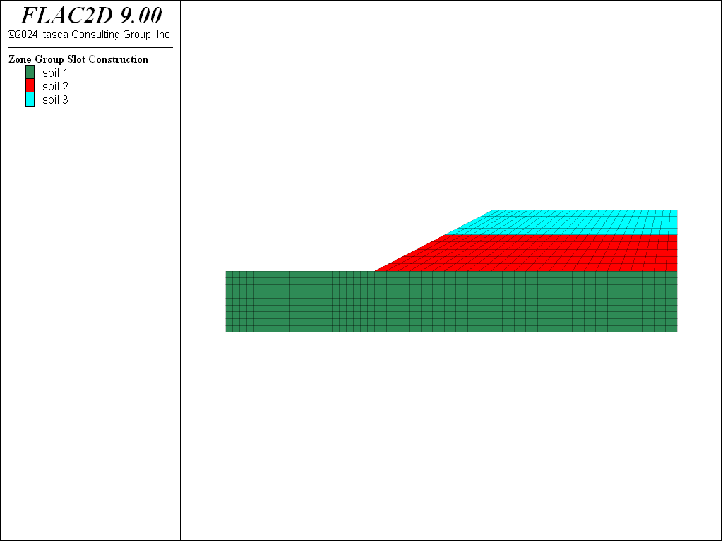
Figure 1: Soil profile.

The liquefiable part of the middle layer is modeled using the P2PSand model and other soils are modeled using the Mohr-Coulomb model plus hysteretic damping.

Several analysis stages are required:

• build model

• setup initial stress and pore-pressure;

• install structures;

• assign P2PSand model; and

• dynamic analysis.

Build Model

A sketch is used to build the model geometry as described in the following steps.

• Create a new sketch set.

• Open the Slope Wizard and enter the parameters as shown in Figure 2

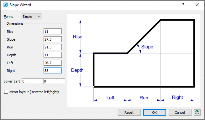
Figure 2: Slope Wizard

• Draw a horizontal line from the toe of the slope to the right side. Draw another horizontal line at \(y\) = 17.5.

• To ensure a structured mesh, draw a vertical line from the toe of the slope to the bottom. The slope should appear as in Figure 3.

Note that when drawing the vertical line, it will attempt to snap to the grid and will create a slightly non-vertical line. This is acceptable, if a perfectly vertical line is wanted, turn off grid snapping for this operation, or manually change the coordinates after drawing the line.

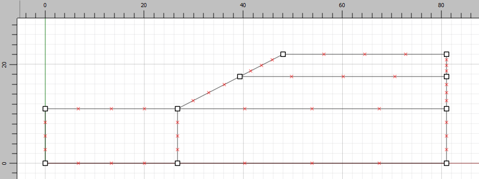
Figure 3: Slope layers

• Set the zone length to 1.25 and mesh all blocks.

• Select the block representing the top layer and assign it the group name “soil 3”. Set the middle layer to “soil 2” and the two blocks comprising the bottom layer to “soil 1”.

• Generate the zones. In the workspace, the model view should appear as shown in Figure 4.

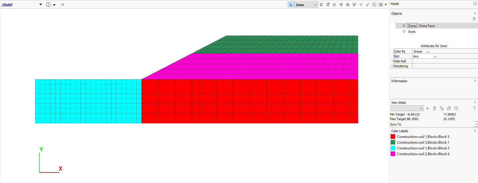
Figure 4: The slope model in the Model Pane.

• At this stage, all soils are Mohr-Coulomb materials. The soil matrix material properties are listed in Table 1. Select the entire model and set the constitutive model to Mohr-Coulomb. Then select each layer and assign the properties as shown in the table. It may help to change the slot of the groups being shown to “Construction”.

Table 1: Soil Properties

Soil	Density	Bulk	Shear	Friction	Cohesion
	Mg/m3	kPa	kPa	deg.	kPa
#1	1.7	5.10e5	2.35e5	40	4
#2	1.5	1.36e5	6.30e4	35	2
#3	1.4	1.36e5	6.30e4	30	2

• Finally, click the icon to “Assign group names to faces automatically”. Check the box to “Ignore existing group names”.

• Save the project and the model state. It is also a good practice to click on the State Record tab in the Commands area aand save the commands as a data file.

Setup Initial Stress and Pore-Pressure

From this point forward, data files are used to perform the analysis. The data files are shown below. This model requires configuring fluid and dynamic analyis (model configure fluid dynamic. At this stage, both fluid and dynamic are off. This model follows the standard boundary conditions: fixed degrees of freedom at the bottom and roller boundaries on the side surfaces. The boundary conditions can be assigned using the face group names created from the Model view in the Workspace.

zone face apply velocity-x 0 range union group 'West' group 'East'
zone face apply velocity (0,0) range group 'Bottom'

The fluid-related material properties are water density \(\rho_f\) = 1e3 \(kg/m^3\), porosity = 0.3. Gridpoints above the water table are set to zero saturation while others are 1 by default. Note that the input soil density should be dry density since fluid is configured.

The pore pressures are initialized by specifying a water table. Static water pressure should be applied to the soil surfaces below the water table to account for the weight of the water. These can be performed by two simple commands:

zone water plane origin 0,20 normal 0,-1
zone face apply stress-normal -200 gradient 0 10 ... 
        range group 'top' position-y -10.99 20

The model is cycled to equilibrium by the command:

model solve elastic convergence 1

Install Structures

This stage sets up the wharf structures.

Before installation of structures, the model should be re-initialized to zero displacements and velocities and be cleared of all yield states because any previously calculated displacement/velocity and yield states are solely provide an initial field of stress and pore-pressure for subsequent stages. These operations are performed with the commands:

zone gridpoint initialize velocity (0,0)
zone gridpoint initialize displacement (0,0)
zone initialize state 0

The platform is modeled by beam elements and the foundations are modeled by pile elements. The thickness of the beam is 0.3 m. The diameter of the piles is 0.6 m. The structure geometry and properties are summarized in Table 2. The friction between the piles and the soil is assumed to be 30 degrees.

Table 2: Structure Properties

Structure	Density	Young	Poisson	Thickness	Diameter
	Mg/m3	kPa		m	m
Beam	2	2e8	0.2	0.3
Pile	2	2e7	0.2		0.6

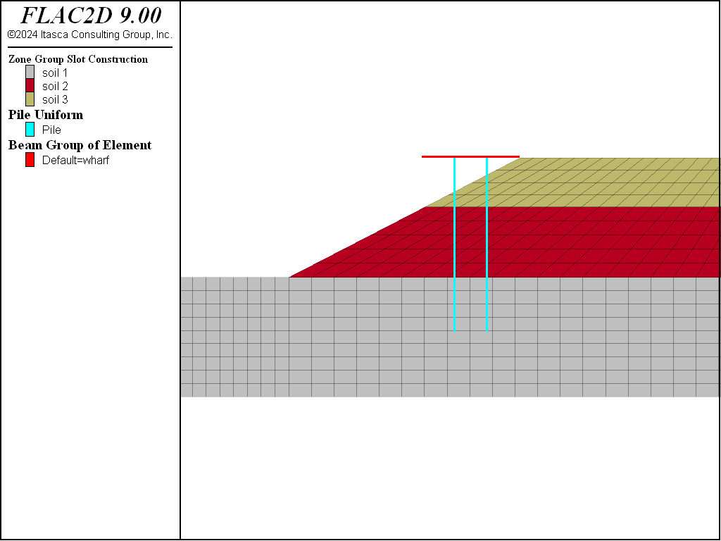
Figure 5: 3D soil profile and schematic of wharf and its piles.

To account for the end-bearing effect of the piles, an additional set of links are created at the pile ends. This is necessary because the default pile links are frictional. If a node requires multiple links, the links can be created on a different ‘side’. In this model, the ‘side=2’ designation is used for end-bearing links (grouped under the name ‘End’) between the piles and the soil. The end-bearing links are assumed to be of the norm-yield type.

Note that the link displacement is defined as the target displacement minus the node displacement. The (downward) driving is regarded as the ‘tension’ of the link, while the (upward) pulling is considered the ‘compression’ of the link. Therefore, the yield-compression of the link is set to zero, while the yield-tension is assigned a large value to ensure consistency with the effect of end-bearing. The commands associated with the end-bearing links are:

structure link create side=2 target zone group 'End' range position-y 5.9 6.1
structure link attach x=normal-yield y=free range group 'End'
structure link attach rotation=free range group 'End'
structure link property x area=[math.pi*d^4/64] stiffness=1e6 ...
       yield-compression=0 yield-tension=1e20 range group 'End'

To make sure the pile heads are rigidly linked to the beam, the following command is used

structure node join range group 'wharf'

Note that there must be coincident nodes to be able to join them.

Again, the model is cycled to equilibrium for the installation of the structures.

Assign P2PSand model

The P2PSand model is applied to certain zones within the middle soil layer (colored by green in Figure 6). To simplify the analysis and demonstration, the internally calibrated material parameters for the P2PSand model are utilized. The primary parameter, relative-density-initial, is set at 0.50 and 0.75 to examine the impact of sand densities on the dynamic behavior of the slope and wharf. The reference pressure is assigned as pressure-reference = 100, as the model’s unit for stress/pressure is in kPa.

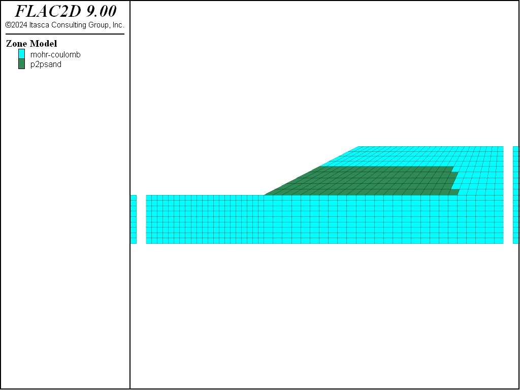
Figure 6: Constitutive models used to represent the soil.

Because the P2PSand model is a stress-dependent model, the initial stress will be utilized to determine the initial moduli. A small FISH function is adopted here:

fish operator ini_stress(z, modelname)
    if zone.model(z) == modelname then
        local pp = zone.pp(z)
        zone.prop(z,'stress-xx-initial') = zone.stress.xx(z) + pp
        zone.prop(z,'stress-yy-initial') = zone.stress.yy(z) + pp
        zone.prop(z,'stress-zz-initial') = zone.stress.zz(z) + pp
        zone.prop(z,'stress-xy-initial') = zone.stress.xy(z) 
    endif
end
[ini_stress(::zone.list, 'p2psand')]

Note that here the keyword operator is used in place of the usual define, declaring it a function to be used with multi-threading. The argument ‘z’ is a zone pointer and ‘modelname’ is a constitutive model name. The command [ini_stress(::zone.list, ‘p2psand’)] runs the FISH function “ini_stress” in a multi-threaded mode.

After assigning the P2PSand model, the model requires another re-initialization of displacement/velocity and yield state to zero. This time, structure nodes require similar re-initialization as well:

structure node initialize displacement (0,0)
structure node initialize displacement-rotational 0

To this point, all necessary constitutive models and structures with allowable stress, pore-pressure, and structural forces forces are set up. The model is ready for dynamic analysis.

Dynamic Analysis

The dynamic configuration needs to be turned on for dynamic analysis. Because the earthquake can be considered a quick loading, the response of the soil is approximately considered an undrained process. To achieve this, fluid calculations are left off (fluid does not flow), but a non-zero fluid bulk modulus is assigned so that changes in pore volume will cause pore pressure changes. The fluid modulus is assigned a non-zero value 2e5 kPa so that the deformation from the soil matrix can cause the change of pore-pressure. Note that a smaller water bulk modulus 2e5 kPa rather than the real water bulk modulus 2e6 kPa is assigned because the water is unconfined—a free surface exists—and likely will be more compressible.

model dynamic active on
zone gridpoint initialize fluid-modulus 2.0e5

The base of the model is considered compliant, so the input motion at the base should be the upward motion, or half of the outcrop motion. The input outcrop motion (labeled Nahanni) before scaling is shown in Figure 7:

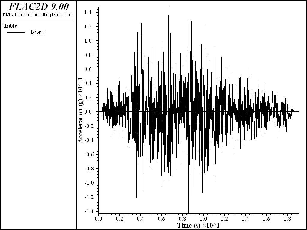
Figure 7: Input acceleration motion before scaling.

Note that the input acceleration in in \(g\) and needs to be multiplied by 10 to convert to m³/s. Also, in practice, the adopted input motion is usually scaled to abide by some design codes or guidelines. In this example, a scaling factor of 5 is used so that the maximum acceleration is around 0.75 g.

At the base, quiet boundaries are used to accommodate the compliant base. The input acceleration motion is integrated into a velocity motion and then into a shear stress history. Shear stress can be calculated from velocity by:

\[\tau = -2 \rho C_s v_{s,upward} = - \rho C_s v_{s,crop}\]

where \(\rho\) is density at the base, \(G\) is the shear modulus at the base, and \(v_s\) is the shear wave velocity, and \(C_s = \sqrt{G / \rho}\) is the speed of s-wave propagation at the base.

The commands are

zone gridpoint free velocity
[table.as.list('vel') = table.integrate('acc')]
[global mf = -1.8*math.sqrt(2.35e5/1.8)*10*5.0]    
zone face apply stress-xy [mf] table 'vel' range group 'bottom'
zone face apply quiet range group 'bottom'

For zones that use the Mohr-Coulomb model, hysteretic damping is incorporated to account for the \(G/G_{max}\) effect. In contrast, zones that use the P2PSand model have an intrinsic energy dissipation in their constitutive relation, so additional energy dissipation is not strictly necessary. However, a small amount of Rayleigh damping is added to zones in order to reduce high-frequency noise. Since the Rayleigh damping is very small, the dynamic timestep is rarely affected.

For structures, the situation is different as the inclusion of Rayleigh damping can significantly reduce the timestep. Therefore, this model uses Maxwell damping with a target damping ratio of 5% for structures (see Maxwell Damping):

zone dynamic damping hysteretic hardin 0.2 range cmodel 'mohr-coulomb'
zone dynamic damping rayleigh 0.0015 1.0
structure dynamic damping maxwell 0.0385 0.5 0.0335 3.5 0.052 25.0

A free-field boundary is then applied following the basic guidelines for dynamic analysis (Free-Field Boundaries).

zone dynamic free-field on

Results

The results for sand \(D_r\) = 0.50 (50%) are plotted in Figure 8 to Figure 10. Figure 8 plots pore-pressure histories at selected points (35,13), (46,14) and (58,15). Apparent excess pore-pressure builds-up are observed. Figure 9 plots the contour of the maximum shear strain. Figure 10 plots the \(x\)-displacement histories of the platform, the slope top, and the base. Interestingly, the lateral displacement of the platform is less than that of the slope, which is a common effect of soil-structure interaction. Specifically, the lateral spreading of the soil pushes the pile foundation, while the pile foundation reinforces the stability of the slope to some extent.

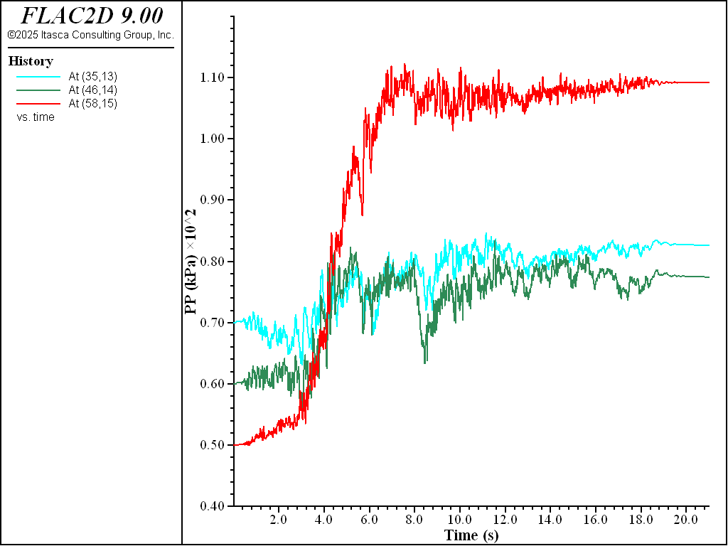
Figure 8: Pore pressure histories for sand Dr = 50%.

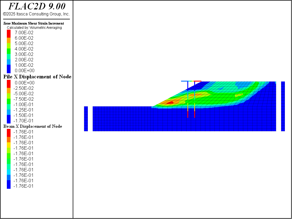
Figure 9: Contour of maximum shear strain for sand Dr = 50%.

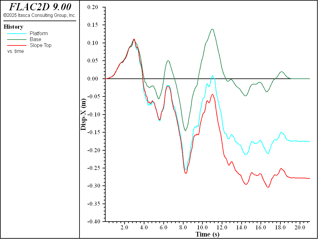
Figure 10: \(x\)-displacement histories for sand Dr = 50%.

Similar results for sand \(D_r\) = 0.75 (75%) are plotted in Figure 11 to Figure 13. Excess pore-pressure builds-up are observed in Figure 11. Lateral displacements of platform and slope shown in Figure 13 are less than those in Figure 10, which is apparently due to the sand in Figure 13 being denser.

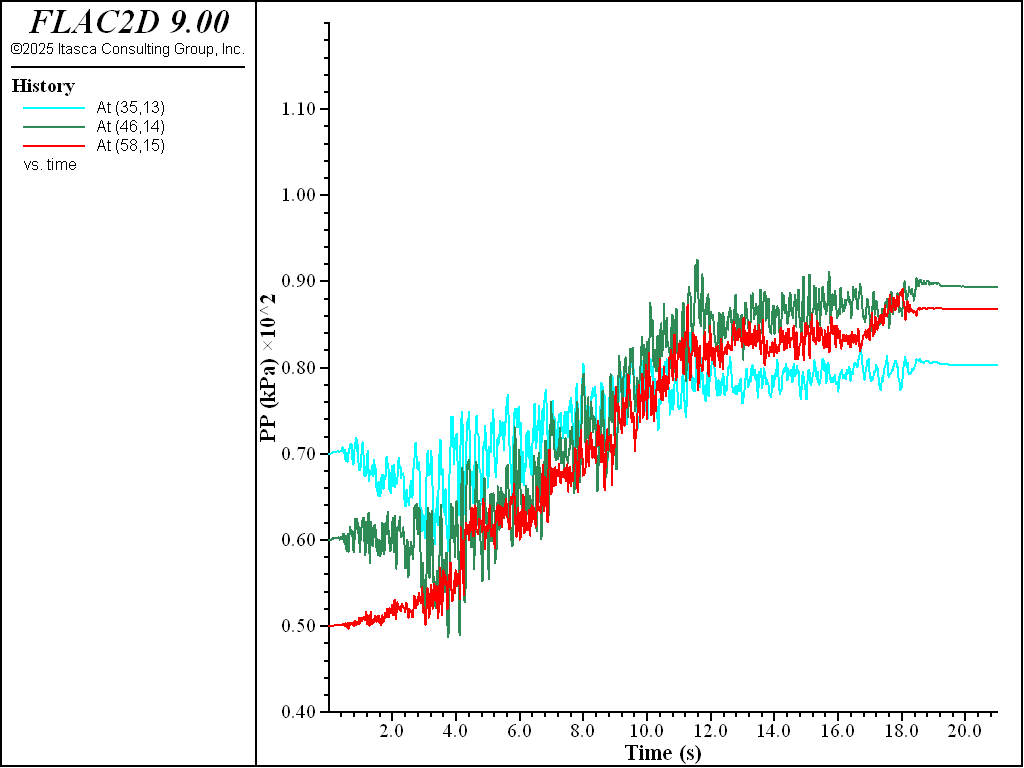
Figure 11: Pore pressure histories for sand Dr = 75%.

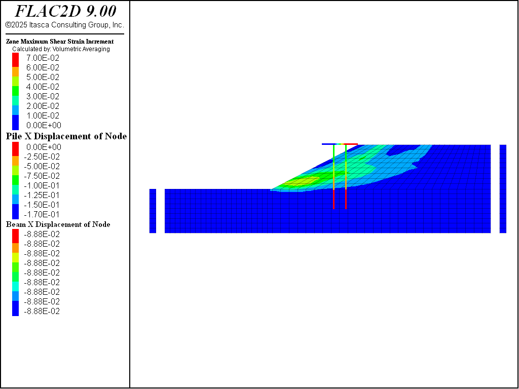
Figure 12: Contour of maximum shear strain for sand Dr = 75%.

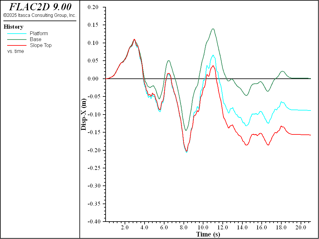
Figure 13: \(x\)-displacement histories for sand Dr = 75%.

break

Data Files

wharf-ini.dat

model new

; Commands from Sketch and Model Pane
program call 'geometry.dat'

model configure fluid dynamic
model large-strain off
model fluid active off
model dynamic active off
model gravity 0 -10
;
zone face apply velocity-x 0 range union group 'West' group 'East'
zone face apply velocity (0,0) range group 'Bottom'
;
; fluid 
zone fluid cmodel assign isotropic
zone water density 1.0
zone fluid property porosity 0.3
zone gridpoint initialize saturation 0 range position-y 20 100

; assume water table is 2 m below the surface (y=20)
zone water plane origin 0,20 normal 0,-1
;zone gridpoint initialize pore-pressure 200 ... 
;        gradient 0 -10 range position-y 0 20
        
; stress applied to the slope to account for the weight of water
zone face apply stress-normal -200 gradient 0 10 ... 
        range group 'top' position-y -10.99 20
;
model solve elastic convergence 1

model save 'wharf-ini'

wharf-struct.dat

model restore 'wharf-ini'

zone gridpoint initialize velocity (0,0)
zone gridpoint initialize displacement (0,0)
zone initialize state 0
;
structure pile create by-line 42,6 42,22.1 segments 8 id 1 reverse
structure pile create by-line 45,6 45,22.1 segments 8 id 2 reverse
;
[global d = 0.6]
structure pile property density 2 young 2e7 poisson 0.2 ... 
    cross-sectional-area [math.pi*d^2/4] ... 
    moi [math.pi*d^4/64] ... 
    coupling-stiffness-shear 1e5 coupling-friction-shear 30 ...
    coupling-stiffness-normal 1e5 coupling-friction-normal 30 ... 
    perimeter [math.pi*d] coupling-gap-normal off
    
; Include end-bearing effect
structure link create side=2 target zone group 'End' range position-y 5.9 6.1
structure link attach x=normal-yield y=free range group 'End'
structure link attach rotation=free range group 'End'
structure link property x area=[math.pi*d^4/64] stiffness=1e6 ...
       yield-compression=0 yield-tension=1e20 range group 'End'
;
; create deck
structure beam create by-line 39,22.1 48,22.1 segments 3 id 3 group 'wharf'
;
; thickness is 0.3 m
structure beam cmodel assign elastic
structure beam property cross-sectional-area 0.3 ...
    density 2 young 2e8 poisson 0.2 ... 
    moi [0.3^4/12.0] range id 3
structure node join range group 'wharf'

model cycle 0
structure node system-local reverse-y range structure-type pile
structure node fix system-local range structure-type pile
;
model solve convergence 1
model save 'static'

wharf-p2p-dr75.dat

model restore 'static'
;
zone cmodel assign p2psand range group 'soil 2' ... 
        position-x 0 70
zone property relative-density-initial 0.75 pressure-reference 100 ... 
        friction-critical 35.0 range cmodel 'p2psand' 
;
fish operator ini_stress(z, modelname)
    if zone.model(z) == modelname then
        local pp = zone.pp(z)
        zone.prop(z,'stress-xx-initial') = zone.stress.xx(z) + pp
        zone.prop(z,'stress-yy-initial') = zone.stress.yy(z) + pp
        zone.prop(z,'stress-zz-initial') = zone.stress.zz(z) + pp
        zone.prop(z,'stress-xy-initial') = zone.stress.xy(z) 
    endif
end
[ini_stress(::zone.list, 'p2psand')]
;
model solve convergence 1

==========================================================
; Dynamic analysis
; 
zone gridpoint initialize displacement (0,0)
zone gridpoint initialize velocity (0,0)
zone initialize state 0
structure node initialize displacement (0,0)
structure node initialize displacement-rotational 0

model dynamic active on
zone gridpoint initialize fluid-modulus 2.0e5
;
; free boundary
zone gridpoint free velocity

; get earthquake history as acceleration
table 'acc' import "Nahanni.acc"

; integrate to get velocity
[table.as.list('vel') = table.integrate('acc')]

; shear stress = -2*sqrt(G/density)*density
; input motion is half of the outcrop motion
; multiplied by 10 to convert from g to m/s2
; multiplied by a scaling factor of 5
[global mf = -1.8*math.sqrt(2.35e5/1.8)*10*5.0]    
zone face apply stress-xy [mf] table 'vel' range group 'bottom'
zone face apply quiet range group 'bottom'
;
zone dynamic damping hysteretic hardin 0.2 range cmodel 'mohr-coulomb'

; 0.15% damping.  Center frequency 1 Hz.
zone dynamic damping rayleigh 0.0015 1.0

; target 5% for structure elements (& transferred to deformable links)
structure dynamic damping maxwell 0.0385 0.5 0.0335 3.5 0.052 25.0
;
zone dynamic free-field on
;
model history name 'time' dynamic time-total
program call 'excpphist.fis'
zone history name 'At (35,13)' pore-pressure source gridpoint position 35 13
zone history name 'At (46,14)' pore-pressure source gridpoint position 46 14
zone history name 'At (58,15)' pore-pressure source gridpoint position 58 15
structure node history name 'Platform' displacement-x position 39,22.1
zone history name 'Base' displacement-x position 50 0
zone history name 'Slope Top' displacement-x position 48 22
;
model dynamic timestep maximum 1.00e-4
model solve time-total 21
;
model save 'wharf_dr75'

Endnote

[1]

This example is listed under the present document title in the i Examples dialog use the menu command Help -> Examples… to access.