Speeding Up Granular Flow Simulations
Note
The project file for this example may be viewed/run in PFC.[1] The data files used are shown at the end of this example.
Introduction
This example demonstrates a few strategies one can use to increase the performance of granular flow models in PFC through simulating the Brazil nut effect. One of the first works focused on the study of granular segregation was undertaken by [Brown1939]. The so-called Brazil nut effect (BNE) was coined by [Rosato1987], who used simulations to demonstrate the effect of larger, and heavier, particles migrating upward through a bed of smaller, and lighter, particles in response to shaking. In fact, the picture is much more complicated, with theoretical and experimental examples of the reverse Brazil-nut effect (RBNE), where larger particles sink to the bottom ([Breu2003]). Unlike the Monte Carlo simulations of [Rosato1987], PFC can be used to track the specific details of particle interactions as they hit one another and/or the enclosing container, helping one to gain insights into the physical system. Note that a relatively large body of research exists investigating this phenomena, far exceeding the scope of this example. There are a wealth of laboratory tests, sometimes contradicting one another, and theoretical models as well as numerical simulations. [Kudrolli2004] presents a review of results for the interested reader. In addition, this example neglects particle wear and air resistance which appear to play important roles in some laboratory tests, along with temperature and humidity. Instead, the BNE will be used as a vehicle to understand some pertinent strategies to effectively speed up granular flow simulations in PFC.
Problem Definition
One challenging aspect of the BNE is that the parameter space of possible configurations impacting the system response is very large. For instance, different regimes of segregation can be observed for different amplitudes and frequencies of shaking, different shaking profiles, different container geometries and different frictional values. For very high frequency shaking the material may be effectively fluidized, while convective flow may dominate at lower frequencies (see [Kudrolli2004]). In fact, it seems that the RBNE often requires fluidization, which means high frequency shaking. Here the BNE and RBNE will be demonstrated with some explanation of pertinent mechanisms present in the PFC models.
The model geometry is defined as a 10 cm diameter cylindrical container filled with two species of balls in the presence of gravity. Balls are perfectly spherical pieces used in PFC; the terms ball and particle will be used interchangeably below. The small ball diameter is 0.6 cm while the large ball diameter is 1.2 cm. The large balls are termed “intruders” as in the literature. Inspired by the experiments of [Breu2003], both the BNE and RBNE are simulated. The model is composed of polypropylene small balls (\(\rho=1.5\) g/cm3) that are placed above glass intruders (\(\rho=2.5\) g/cm3). All balls are generated without overlap and gravity is present. While shaking, the difference of the average intruder height to the average small-ball height is recorded and termed the intruder elevation. This measure can be taken as a measurement of intruder migration, with a value of 0 meaning that the intruders are, on average, entrained in the center of the small-ball bed. A number of works demonstrate that friction, especially wall friction, plays an important role in the BNE. Friction exists in the model (\(\mu = 0.6\)). Note that since contact detection parameters are modified later, the normal force is incremental (lin_mode = 1 in the contact model).
Damping is a complex issue for granular flow simulations; see a brief discussion here. One might introduce a small amount of viscous damping based on a coefficient of restitution and the results of this verification problem, for instance. One might also use a small amount of local damping which would speed up the computation as viscous damping decreases the timestep slightly, though local damping is non-physical. The choice of damping depends strongly on the problem. Viscous damping is chosen here corresponding to a coefficient of restitution of ~ 0.9 in the normal direction; the shear viscous damping coefficient is set to the same value as in the normal direction.
The period and amplitude of shaking appear to fundamentally impact the intruder behavior. In addition, it has been observed in these simulations that the shaking time history (i.e., purely sinusoidal velocity versus smoothly varied to the nominal value) impacts the details of the response. The figure below shows one period of the wall velocity imposed in these simulations. This type of time history is smooth and reduces the amplitude of shaking required for segregation, making the segregation less energetic. This is advantageous when trying to understand physical mechanisms responsible for the segregation. Note that the shaking must be vigorous enough that the balls move relative to one another, leaving the floor of the container. Both the frequency and amplitude are changed to demonstrate their influence.

Figure 1: Wall velocity time history with peak amplitude 1 m/s, or 100 cm/s, and frequency 1 Hz, or 1 second period.
As with all granular flow simulations, it is highly advisable to run an ensemble of models composed of different particle packings. In this example, 3 realizations are run simultaneously for each set of model parameters to assess the range of model responses. Of course, 3 realizations is a very small sample size for meaningful statistics, and is likely inadequate for a defensible analysis; it is chosen for computational efficiency here. For each realization there are about 1200 small balls and about 70 intruders. The figure below shows the initial model geometries prior to shaking.
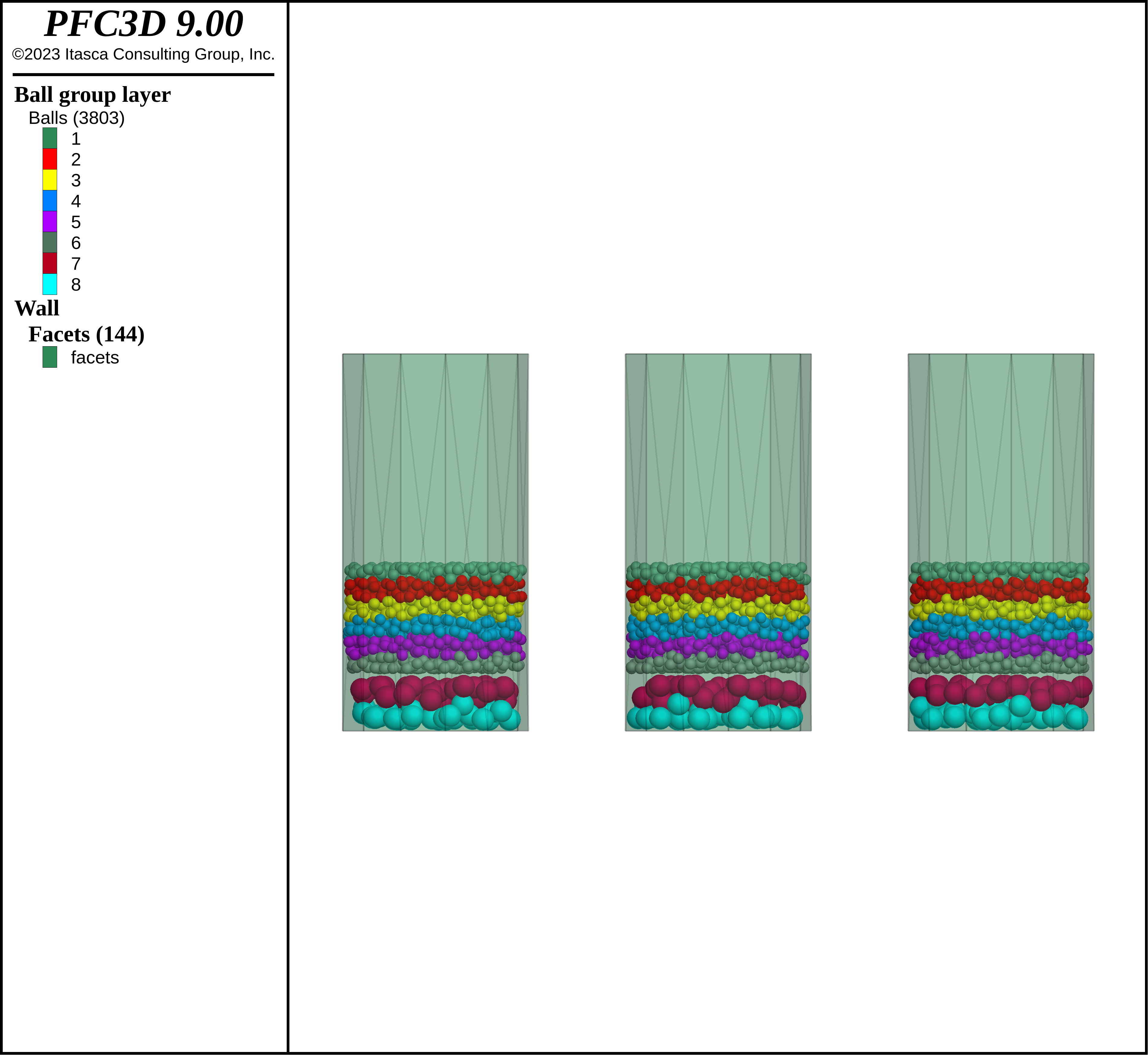
Figure 2: Three realizations of small balls generated above intruders. The intruders are larger (1.2 cm diameter versus 0.6 cm) and more dense (\(\rho=2.5\) g/cm3 versus \(\rho=1.5\) g/cm3) compared with the small balls.
One goal of this example is to gain some physical insights into the mechanisms responsible for BNE and RBNE. As the model is rather simple with few parameters, it is interesting to investigate if gravity, friction and damping, along with sufficient shaking, can produce the effect, and if these simple models seem to point to clear physical explanations. Another goal is to understand what steps may be taken to reduce computational effort. Specifically, this example discusses particle size upscaling, decreasing stiffnesses, fixing the timestep and relaxation of contact detection constraints.
Particle Upscaling
Many granular flow simulations often seek to gain insights into problems comprised of many millions, billions, or even trillions of individual particles. PFC has been used to successfully simulate models ranging from caldera collapse and landslides to powder mixing and tablet compaction, in spite of the fact that model sizes are limited to less than 10 million balls for most practical purposes. It is often not feasible computationally to tackle such problems by modeling each individual particle, regardless of the computational resources available. Frequently one either restricts the volume of material to be modeled considerably or particles are upscaled. Particle upscaling, or coarse graining, is the process of increasing particle sizes, sometimes by more than a few orders of magnitude, while retaining the bulk physical response. In order to gain sensible results, though, upscaled models must be calibrated against known physical tests. [Lommen2019], and references therein, demonstrate some approaches to upscaling particle sizes, resulting in predictive numerical models with reasonable computational durations. In nearly all cases, upscaling requires calibration with a number of laboratory scale tests, such as angle of repose tests, shear box tests, hopper flow tests, etc. In this specific problem, the number of balls is very small and fixed, so particle upscaling is not a feasible method for improving the model performance. When upscaling particles one must also think about the pertinent model dimensions relative to the particle sizes. If the goal is to model a layer of balls in the container, as in this problem, it is advisable that a ball layer has roughly 8 or more balls across the dimension of the container. This same logic applies to having balls flow through orifices, as balls that are too large may jam unrealistically due to hitting the model boundaries. Thus, another important consideration to particle upscaling involves assessing the smallest features of your model boundaries/geometry that may be impact the model response; if particles are large compared to such features then one cannot expect the model to capture the response adequately.
Decreasing Stiffnesses
This examples uses the Linear Model; this is a reasonable choice as we are assuming that the particles are perfect spheres without wear. As none of the theoretical models developed to predict the BNE/RBNE depend on stiffness of the material in question (i.e., [Hong2001]), it is anticipated that the presence of the effect should be relatively insensitive to the stiffness. No stiffness contrast is applied to the different species, only the density and size differences. That being said, too low a stiffness may lead to undesirable effects.
As the shaking is dynamic, using the actual stiffness would result in a rather small timestep. The timestep is dominated by the stiffest and smallest particles in the system. Glass has a Young’s modulus between 50-90 GPa, much stiffer than the polypropylene (1-2 GPa). Assuming a 50 GPa Young’s modulus for the intruders, one can estimate roughly the normal stiffness based on Equation (17) to be about 4.7e8 kg/s2. An intruder with four contacts would result in a timestep around 9e-7 s/cycle using Equation (10), using the default timestep safety factor of 0.8. If the simulation were run for 10 s of real time, this would result in roughly 11 million cycles. Even if the simulation can perform 2,500 cycles per second, it would require more than 74 minutes to simulate this simple system composed of very few balls. Now imagine simulating the granular segregation of a glass powder with millions of particles.
As a side note, since friction is involved, one must set the shear stiffness. As mentioned in [Coetzee2020] and referenced therein, many granular flow simulations set the normal and shear stiffnesses equal; this approach is adopted in the current example.
How important is the stiffness for any particular granular flow problem? How low can it be set and still provide meaningful results? How much speedup can be gained by changing the stiffness? The answers to these questions depend on the details of the problem and what measured quantities are of importance. For instance, [Coetzee2020] showed that for spherical particles, scaling the stiffness down by a factor of 10 and 100 did not change draw down test results appreciably; those tests with scaled stiffnesses were found adequate to calibrate spherical particle models that were then used to predict the responses of additional physical tests successfully. Most simulations reported in the literature scale the stiffness down by factors of 10 to 1,000, with successful results shown for scale factors of even 10,000 [Yan2015].
How much does scaling impact run times? Using Equation (10) once again, the timestep using a stiffness of 1e-7 kg/s2, 1e-6 kg/s2, 1e-5 kg/s2, 1e-4 kg/s2 and 1e-3 kg/s2 would be approximately 2e-6 s, 7e-6 s, 2e-5 s, 7e-5 s and 2e-4 s, respectively. Thus, for each order of magnitude that the stiffness decreases, the timestep increases by a factor of about 3 (i.e., \(\sqrt{10}\)). Said another way, if the goal is to simulate a system for a fixed amount of time, changing the stiffness by an order of magnitude will result in the model taking roughly 1/3rd the amount of time to complete. Scaling the stiffness down by 2 orders of magnitude results in an order of magnitude decrease in the simulation time, all things equal. It is clear that if the pertinent model outputs are insensitive to stiffness then it is highly advisable computationally to scale the stiffness down as much as possible.
Even for this very small model, running with the actual stiffness takes longer than a user might be inclined to wait, especially for an example application. In addition, as the literature points out, scaling stiffnesses down by a factor of 10-1,000 is standard practice. One could take different approaches to verify that modifying stiffness changes do not impact model state, usually involving a restricted model geometry and restricted cycling time. Here, the small particle bed size is reduced and only one layer of intruders is simulated (see the figure below). The intruder elevation is monitored as a function of stiffness and the model is cycled for 2 seconds when shaken by a 10 Hz velocity profile with peak amplitude of 35 cm/s.
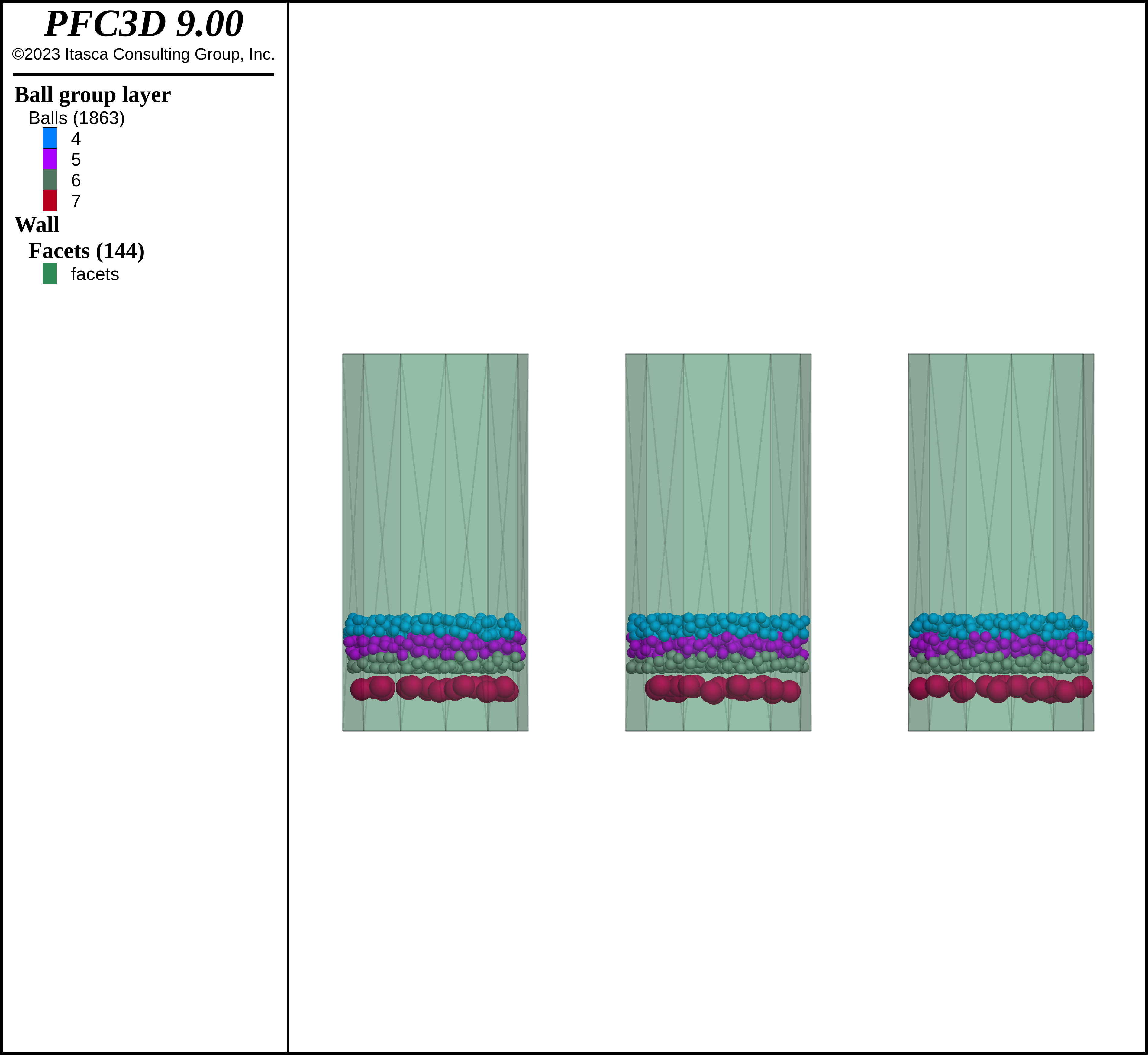
Figure 3: Restricted model used to test model response with changes in stiffness.
The mean intruder elevation, taken over the 3 models, is shown below as a function of time. As one can see, the model responses are different. In particular, the lowest stiffness levels show more rapidly increasing intruder elevation compared with the stiffest response. Given the spread of the highest stiffness elevation time histories, it seems that stiffnesses larger than 1e5 kg/s2 are consistent. One should run more realizations and obtain statistical measures of the differences as a function of stiffness, though such an effort is beyond the scope of this example.
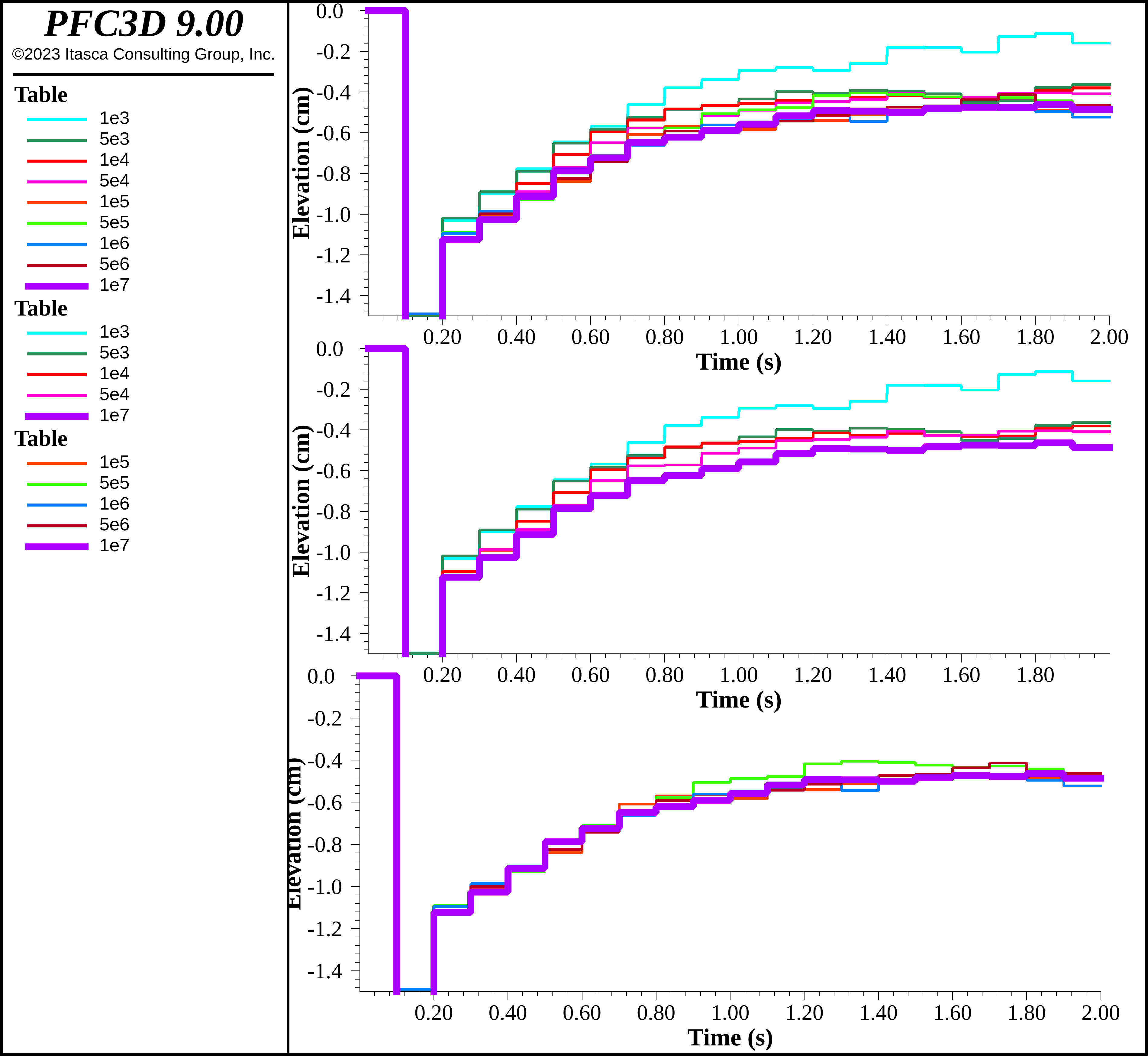
Figure 4: Mean intruder elevation, for different levels of stiffness, as a function of time. The top axis shows all stiffnesses, the middle axis shows stiffnesses 1e3, 5e3, 1e4, 5e4 and 1e7 kg/s2, while the bottom axis shows stiffnesses 1e5, 5e5, 1e6, 5e6 and 1e7 kg/s2.
The table below shows the simulation times for each stiffness level for a specific machine with a 10 core CPU in Linux. All plots were closed and other applications as well, in an effort to accurately measure the running times. If timing is sought it is very important to either set the plot interval to a very large value or close all plots, otherwise plotting time may influence the timing results. There are very few balls and contacts in these models, meaning that the CPU is not running at a high percentage all of the time. Timing tests are most informative when tun on larger models. Operating system interruptions may be reflected in the run times below as well. The number of cycles is sensitive to other computational issues such as the contact detection strategy, as discussed below.
Stiffness (kg/s2) |
Time (s) |
Cycles |
|---|---|---|
1e7 |
496 |
1090186 |
5e6 |
379 |
814554 |
1e6 |
206 |
412409 |
5e5 |
161 |
307700 |
1e5 |
92.4 |
156272 |
5e4 |
70.1 |
117105 |
1e4 |
42.8 |
59197 |
5e3 |
34.1 |
43935 |
1e3 |
21.3 |
22088 |
Modifying the Timestep
The overhead involved computing the stable timestep is not negligible. How can changing the timestep computation scheme be used to decrease the run time? Often, modelers take a trial-and-error approach, fixing the timestep to different values while recording the model response using the model mechanical timestep fix command. One rational approach is to run a small yet representative model, tracking the timestep, and choosing a stable timestep based on those simulations. Another approach is to change the timestep safety factor (see model mechanical timestep safety-factor) to a larger value as the default is 0.8, meaning that the timestep is 80% of the stable value computed.
It is very important to note there is an order dependency to changing the timestep computation mode as a model clean is automatically called when modifying the timestep computation mode, creating contacts if pieces are in proximity; if one of the commands above is given before the contact cmat default model then the Null Model is assigned if pieces are close enough for contacts to be created. One should call the contact cmat apply command after the CMAT is assigned, or should wait to change the timestep computation scheme until the simulation starts. This is the case for the model mechanical timestep scale and model mechanical timestep auto commands as well.
It is crucial to set the timestep correctly as, if the timestep is too large, the model will likely become unstable. This is remediated, to some degree, as the normal force computation is incremental. Modifying the timestep computation scheme is dangerous, but may decrease the run time substantially. The figure below shows the timestep for the a stiffness of 1e5 kg/s2 where the history interval has been set to 1 (see history interval). The timestep ranges from 0.6e-5 s to 2e-5 s, a spread of a factor of more than 3. This is a very dynamic problem; many granular flows show much less variation in timestep. The timestep is variable due to the fact that the contact configuration changes substantially during the rise and fall of the ball assembly.
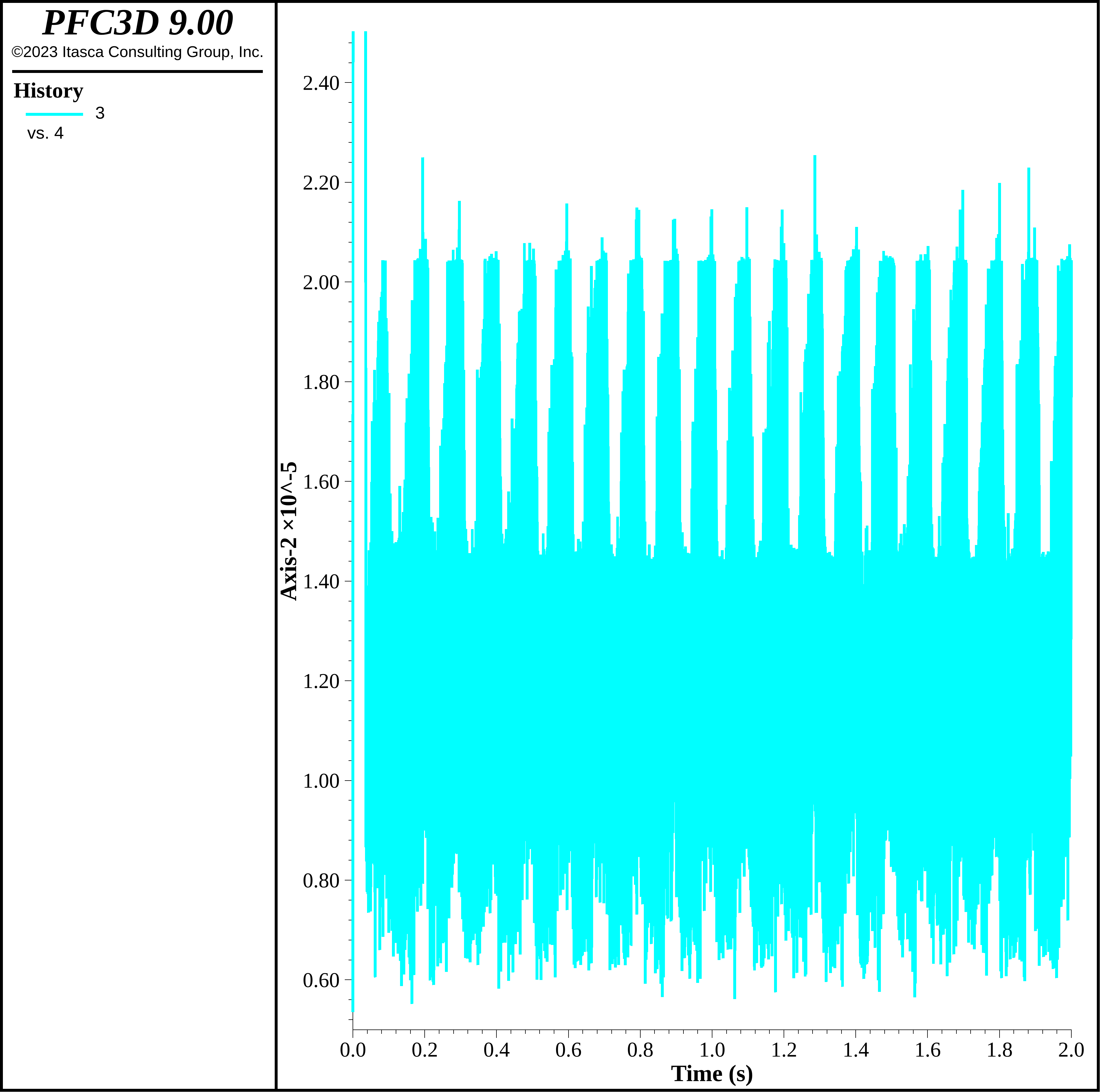
Figure 5: Timestep during the stiffness test using 1e5 kg/s2 stiffness and a history interval of 1.
The figure below shows the intruder elevation with changes in the timestep, both fixing it (to values 8e-6 s, 1e-5 s, 1.2e-5 s, 2e-5 s and 3e-5 s) and for changing the timestep safety factor to 0.9 and 1.0 relative to the default settings. The table below shows the run times and number of cycles for each scenario. As can be observed, the model response are relatively insensitive to the timestep schemes up to perhaps 2e-5 s. The 3e-5 s model produced a substantially different response, though. Modifying the safety factor has a moderate impact on run time, on the order of 10%. Choosing a rather large timestep, such as 2e-5 s, can have a much larger impact, though the timestep must be chosen wisely. The model results below present both the automatic scheme and using a timestep of 2e-5.
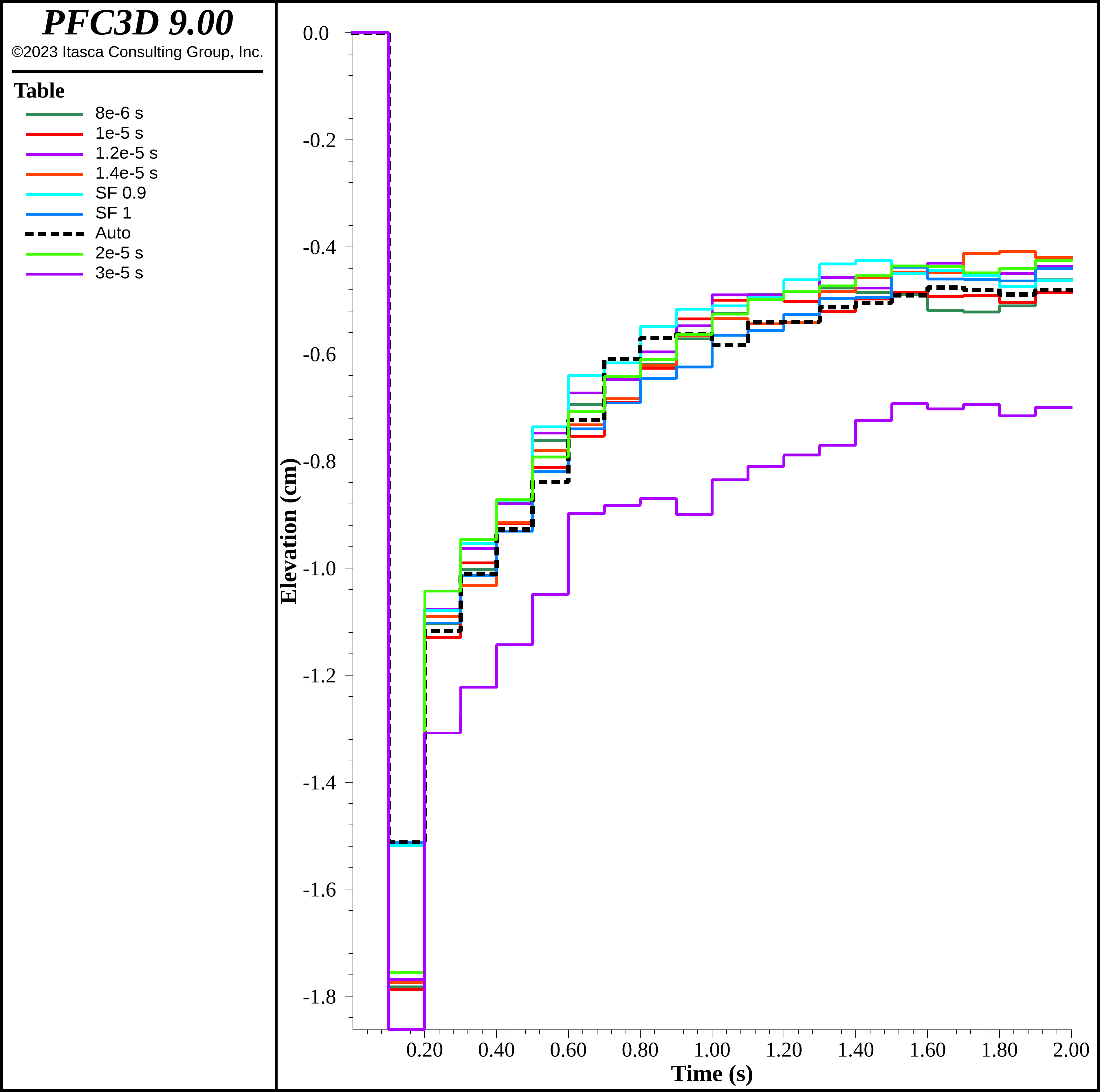
Figure 6: Intruder elevation using 1e5 kg/s2 stiffness. Fixed timesteps of 8e-6 s, 1e-5 s, 1.2e-5 s, 1.4e-5 s, 2e-5 s and 3e-5 s are shown, along with timestep safety factors of 0.9 and 1.0.
Method |
Time (s) |
Cycles |
|---|---|---|
Auto |
92.4 |
156272 |
Timestep fixed 8e-6 s |
128 |
250000 |
Timestep fixed 1e-5 s |
105 |
200000 |
Timestep fixed 1.2e-5 s |
92.7 |
166667 |
Timestep fixed 1.4e-5 s |
80.1 |
142858 |
Timestep fixed 2e-5 s |
57.3 |
100001 |
Timestep fixed 3e-5 s |
39.4 |
66667 |
Safety Factor 0.9 |
85.9 |
141217 |
Safety Factor 1 |
81.0 |
129092 |
Model Results - Convective Regime
With the decision to use 1e5 kg/s2 stiffnesses, the example continues by simulating shaking of the whole ensemble of particles in a convective regime. In this case a 10 Hz velocity profile with 35 cm/s peak amplitude is simulated equivalent to the time history shown above. Groups have been assigned to layers initially, and additional groups are set each time a save file is created, to investigate the segregation characteristics. The figure below shows the intruder elevation for 20 seconds of shaking. Though the intruders are larger and more dense they rise from the bottom of the container. In addition, the rate of elevation increase slows substantially. The simulation time was ~ 32.7 minutes. It is interesting to notice the spread in response as a function of time for the three particle packings, highlighting the necessity to run multiple realizations. These results use the automatic timestep scheme.
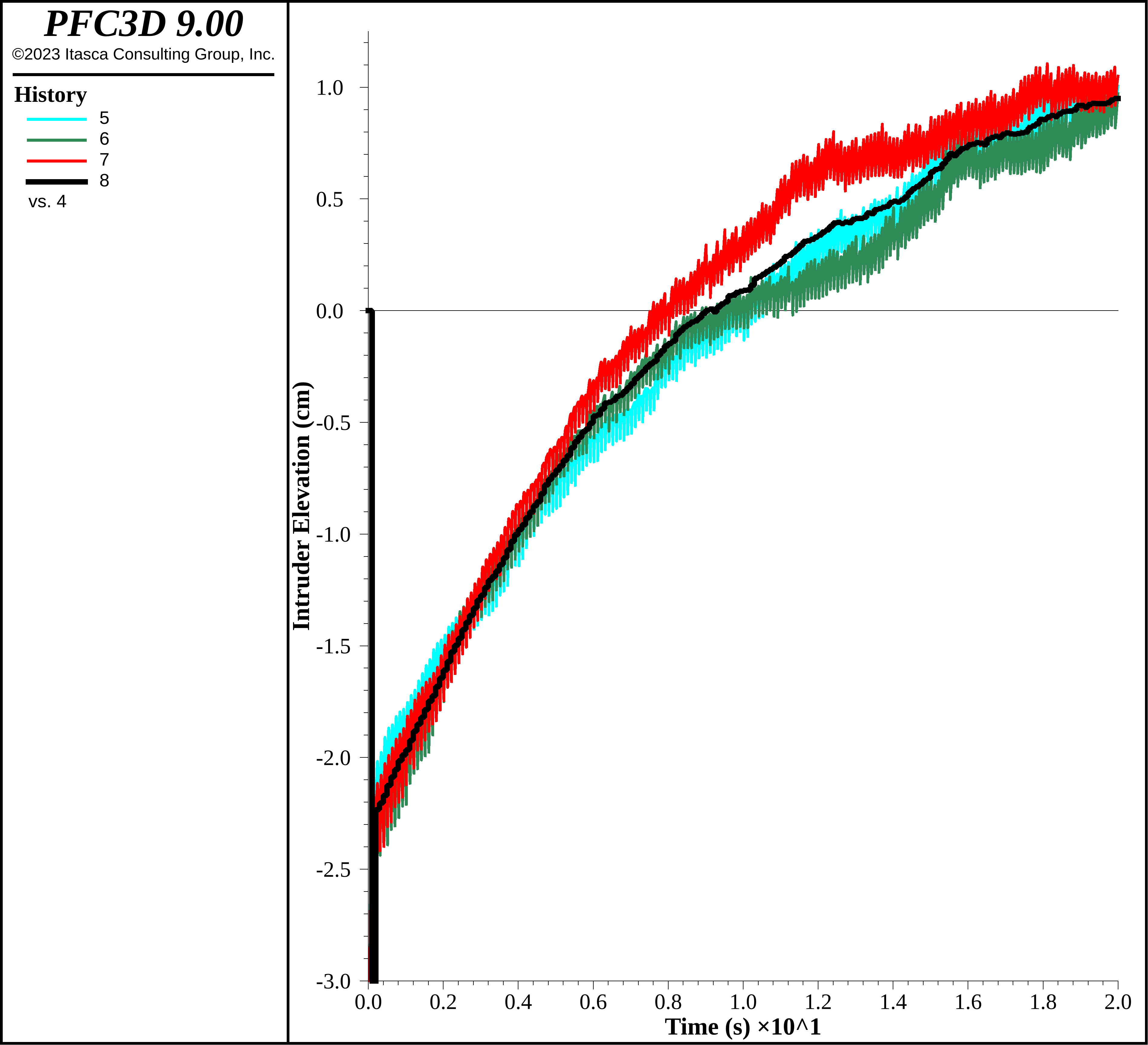
Figure 7: Intruder elevation for 20 seconds of 10 Hz / 35 cm/s shaking.
How are the larger / more dense intruders brought to the surface? Two methods have been employed to understand this behavior, namely particle traces and grouping in layers. Particle traces record the position and velocity of balls as a function of time, with the ability to render the trajectories of the particles. For each model, 3 intruders at the bottom of the assembly and 3 small balls at the top of the assembly are monitored. Results are shown in the figures below. It is evident that some small balls near the top move to the vertical container boundaries (VCBs) and down; subsequently some move toward the center and up, making a clear convection loop. It is also apparent that the intruders closer to the VCBs move in toward the center and up, while the intruders in the center region move primarily up.
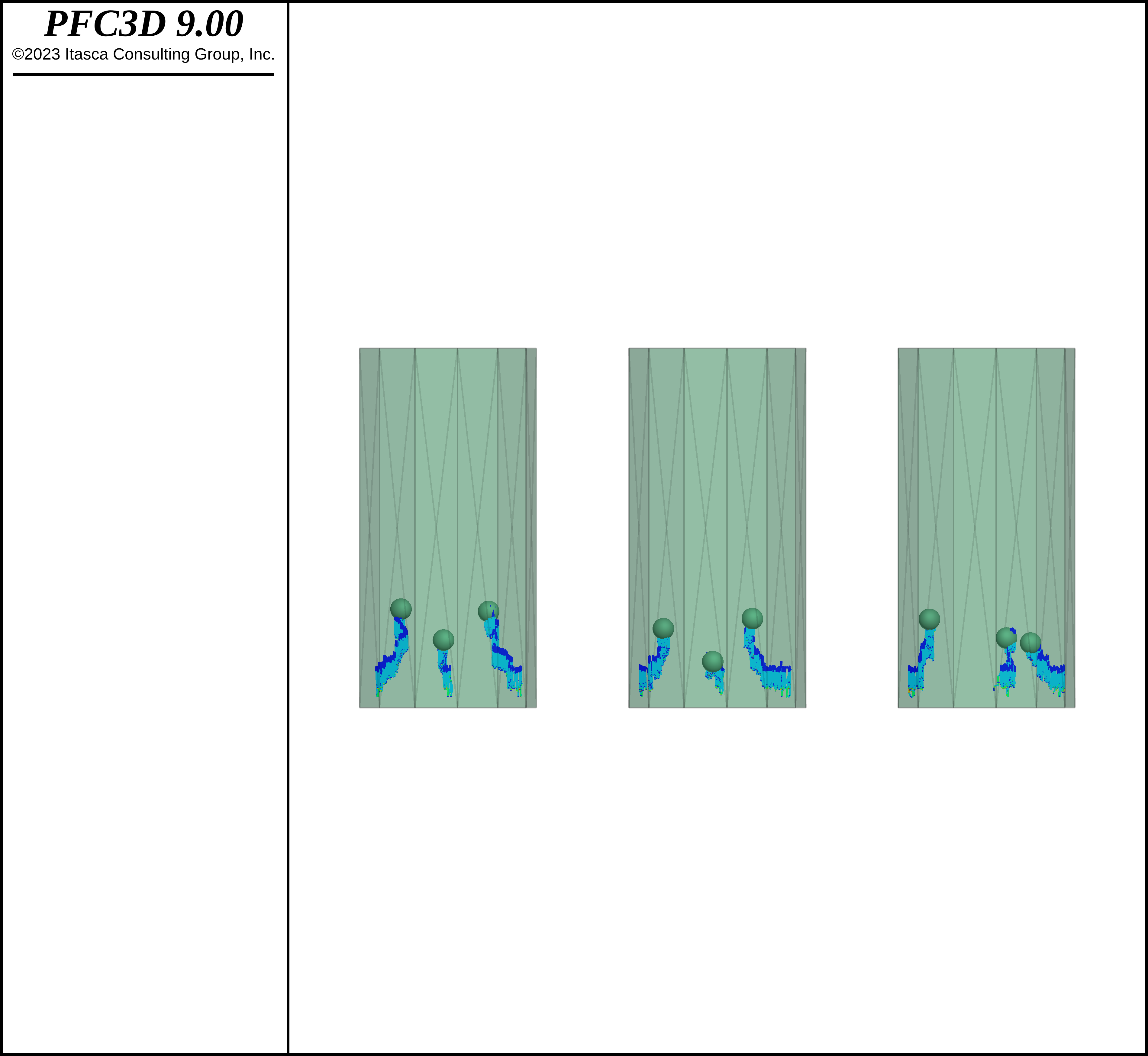
Figure 8: Particle traces (i.e., position and velocity) as a function of time for 3 intruders in each realization.
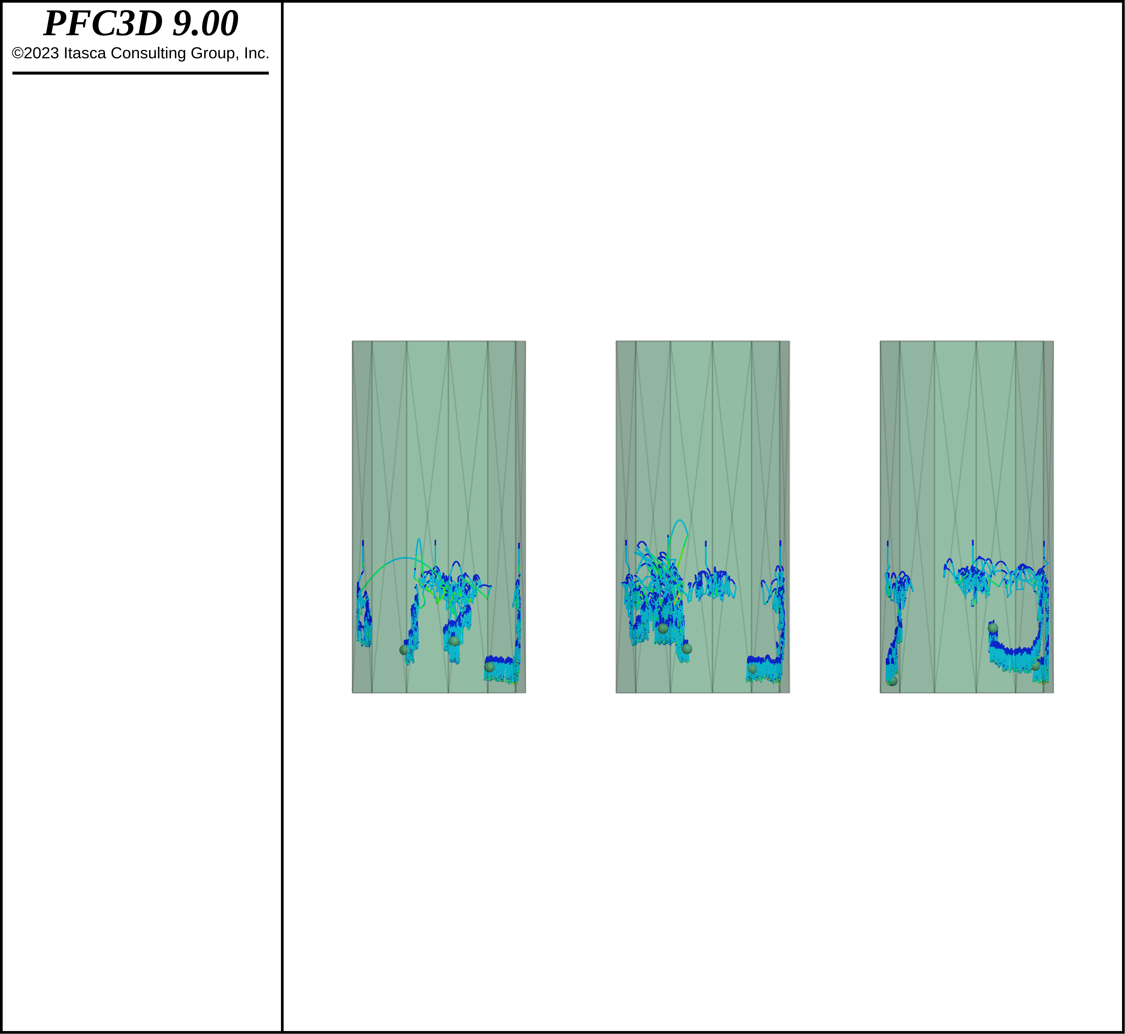
Figure 9: Particle traces (i.e., position and velocity) as a function of time for 3 small balls in each realization.
The figures below show snapshots of the small-ball layer initially at the top of the model for various times. It is clear that this layer progressively moves down along the VCB, thinning above the center of the model. In addition, the figures depict all intruders. This current of small balls moving down is responsible for pushing the intruders into a heap in the center of the model, increasing the thickness of the intruder layer. Eventually the intruders reach the top of the assembly and spread over the top of the small balls; they are largely not able to move down along the VCB, stopping the convection. This is largely the reason that the rate of elevation increase slows as the simulation progresses.
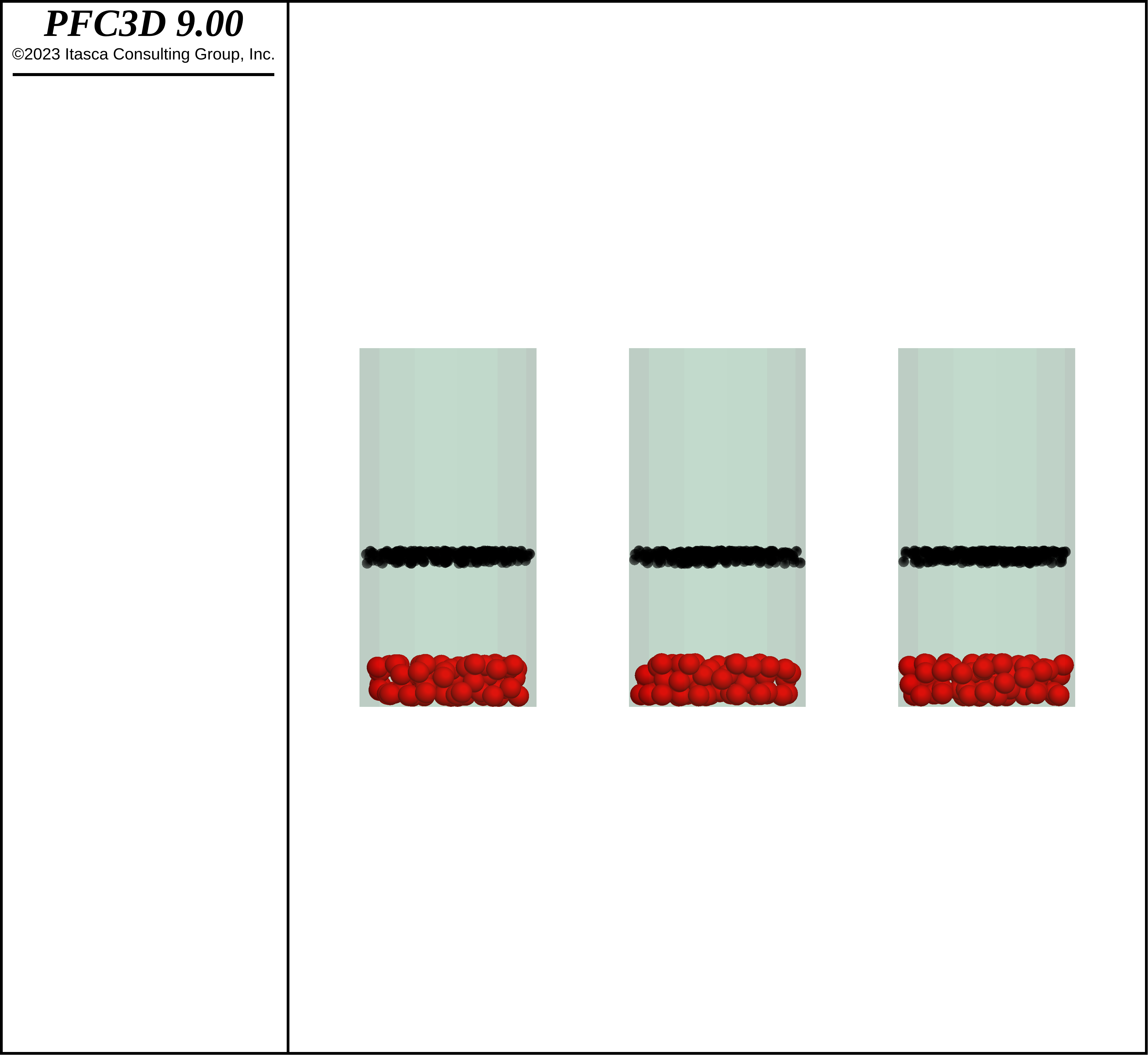
Figure 10: Intruders and top layer of small balls at time 0 s.
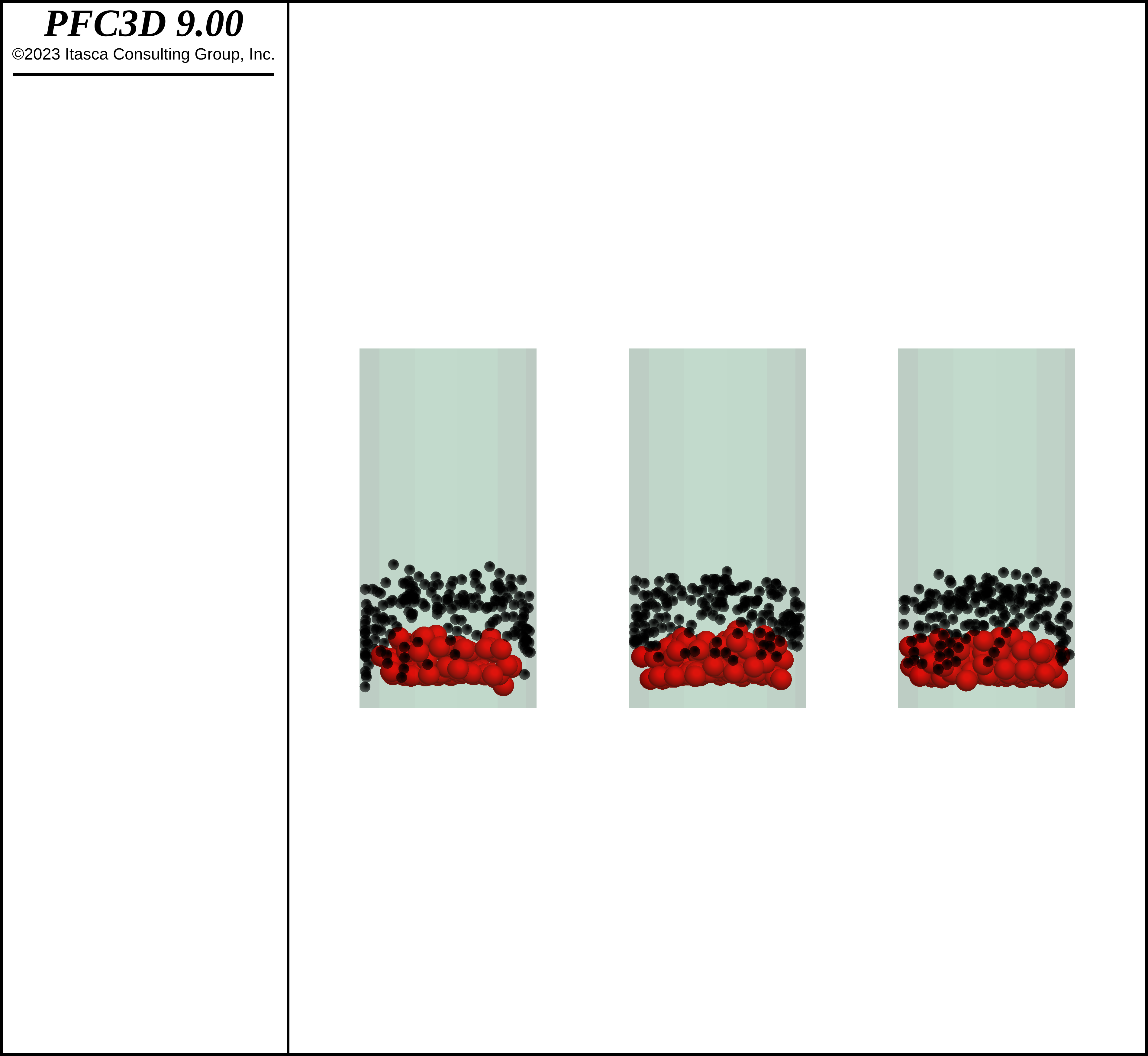
Figure 11: Intruders and top layer of small balls at time 2 s.
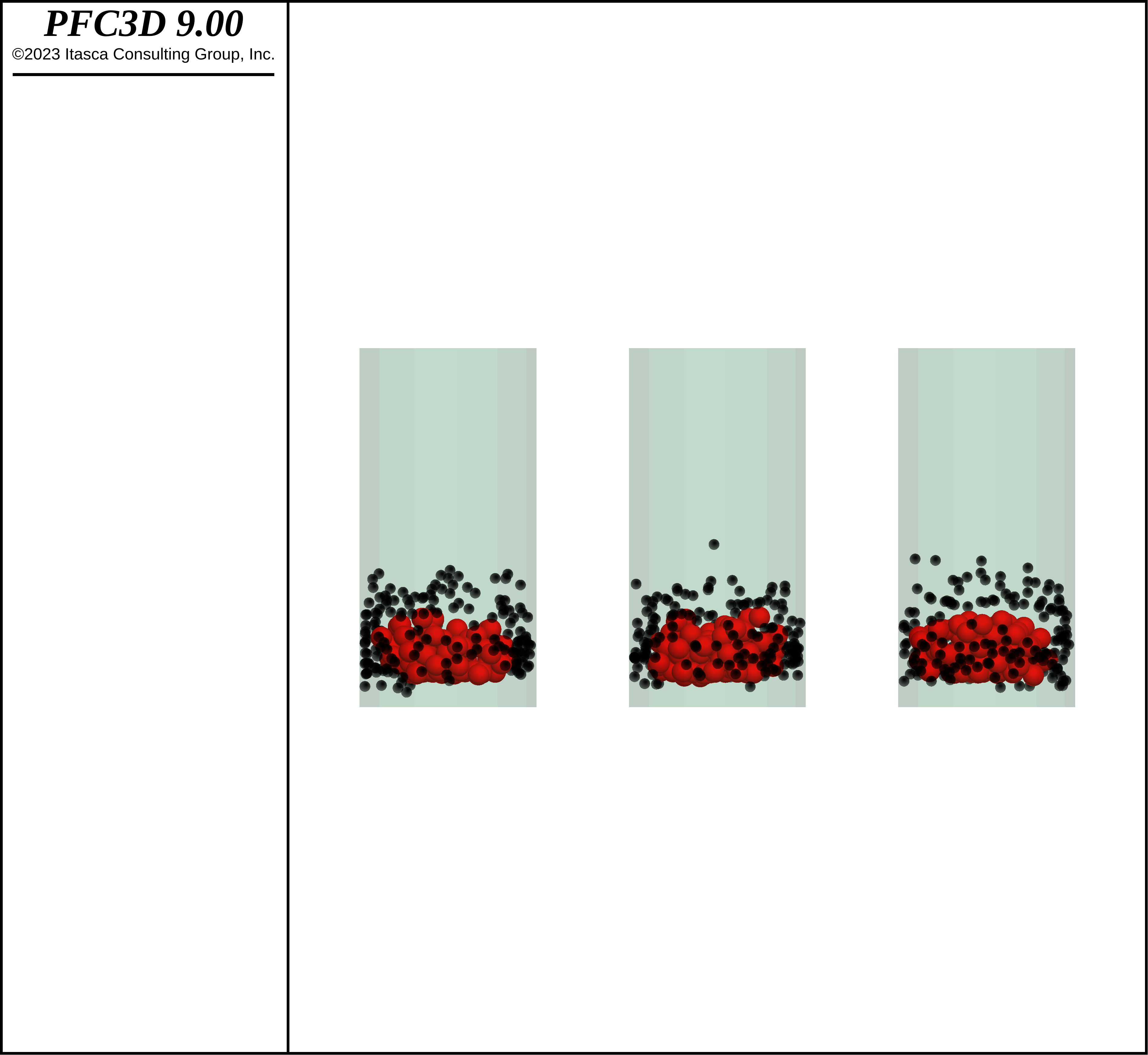
Figure 12: Intruders and top layer of small balls at time 4 s.
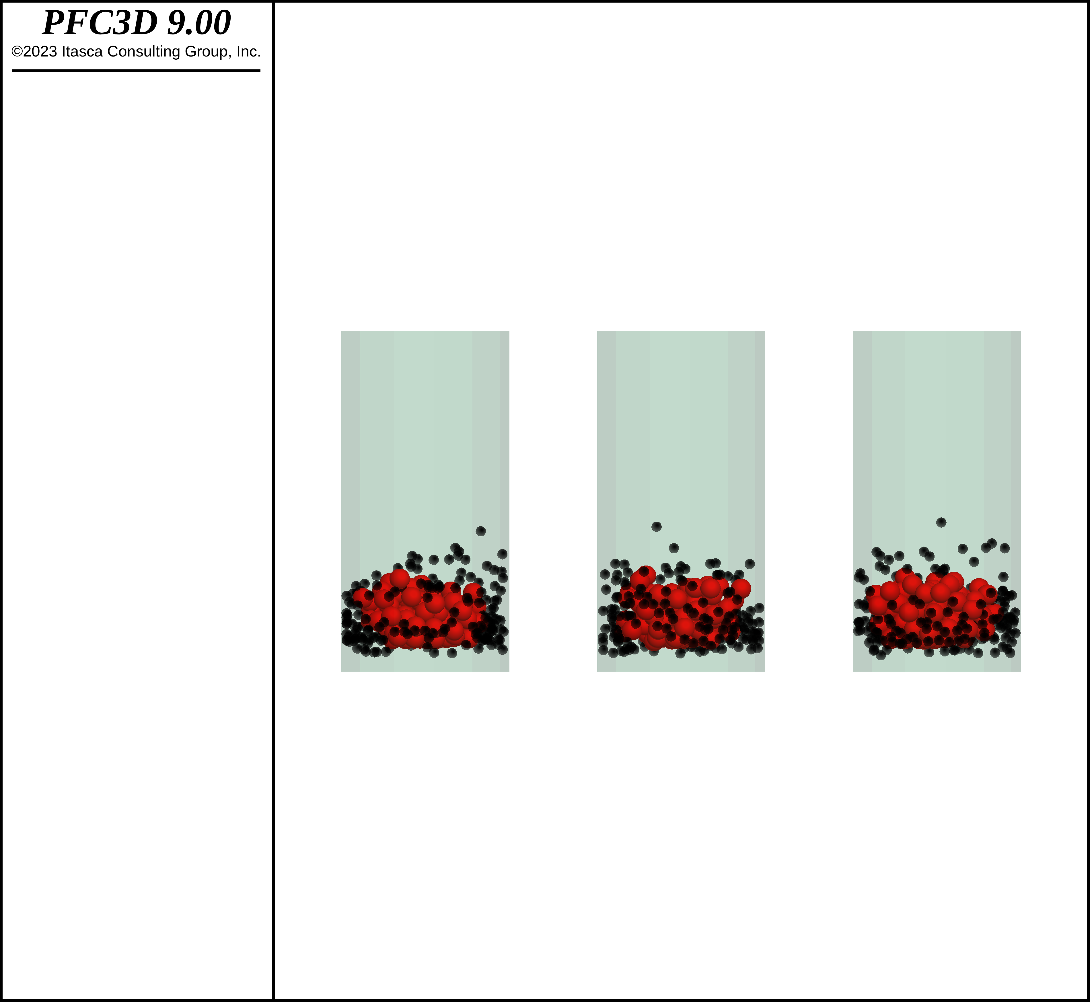
Figure 13: Intruders and top layer of small balls at time 6 s.
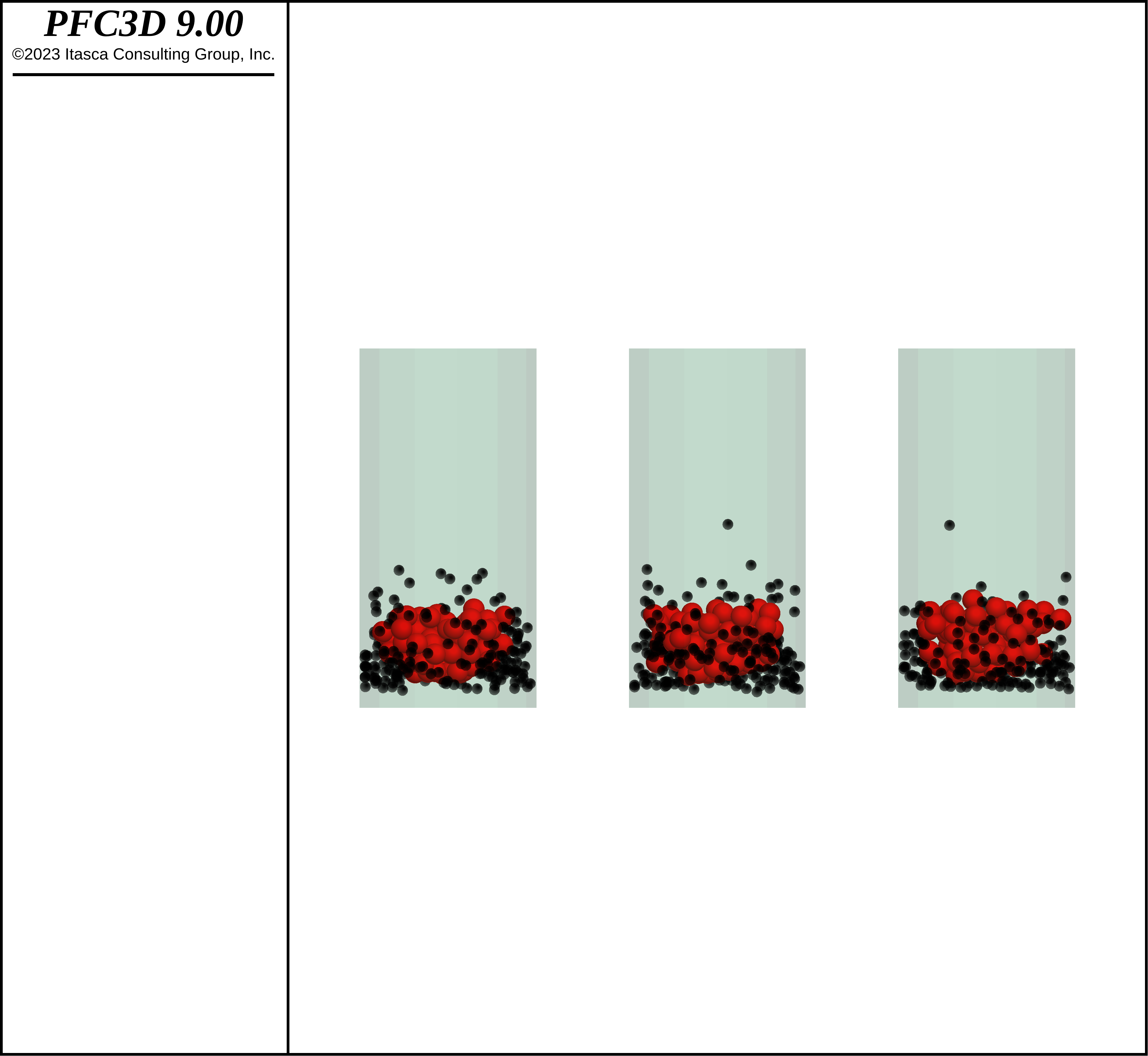
Figure 14: Intruders and top layer of small balls at time 10 s.
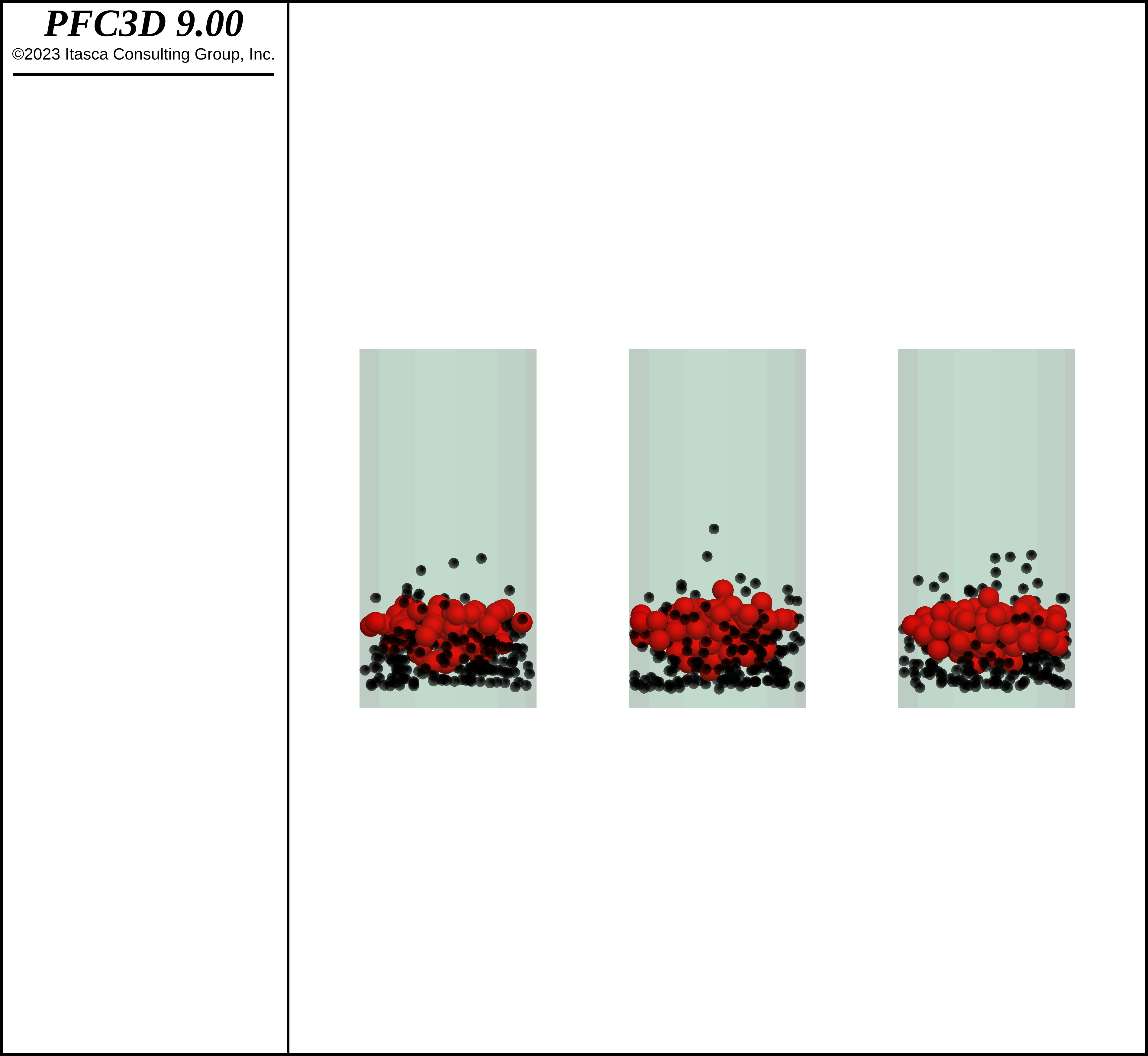
Figure 15: Intruders and top layer of small balls at time 20 s.
These results indicate the the wall friction is an important factor leading to the BNE in this convective regime. As the container moves up, the balls near the VCBs experience more resistance to vertical motion compared with balls away from the VCBs; they represent immovable frictional boundaries that drastically impact the response of the system. The figure below shows the intruder elevation after 5 seconds of shaking with no friction on the VCBs. The BNE in this convective regime has been effectively eliminated.
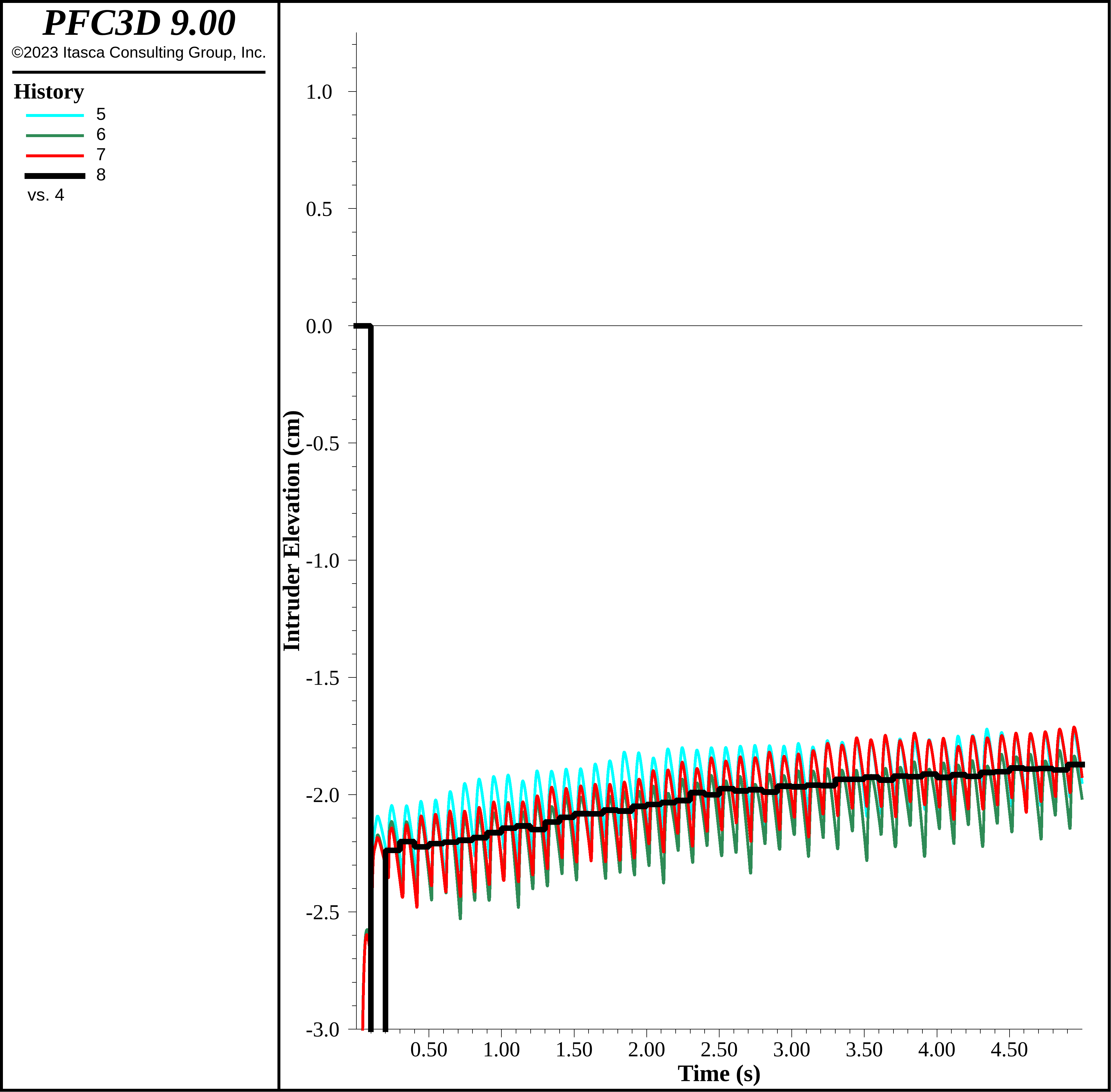
Figure 16: Intruder elevation in the convective regime with 0 wall friction.
Model Results - Fluidized Regime
After 20 seconds of shaking with the 10 Hz / 35 cm/s velocity time history, the frequency is increased to 100 Hz and velocity amplitude increased to 120 cm/s, and shaken for an additional 20 seconds. This high-frequency shaking has a pronounced effect on the system as shown in the intruder elevations below. Though the intruders are initially largely above the small-ball bed, they rapidly begin to descend as the packing has become effectively fluidized; the intruders, of larger size and density, cannot remain buoyant in this regime. Just as some small balls are caught above the intruders in the convective regime, some small balls are caught below the intruders in this regime, so that the intruders cannot completely come to rest at the bottom of the container. These results use the automatic timestep scheme.
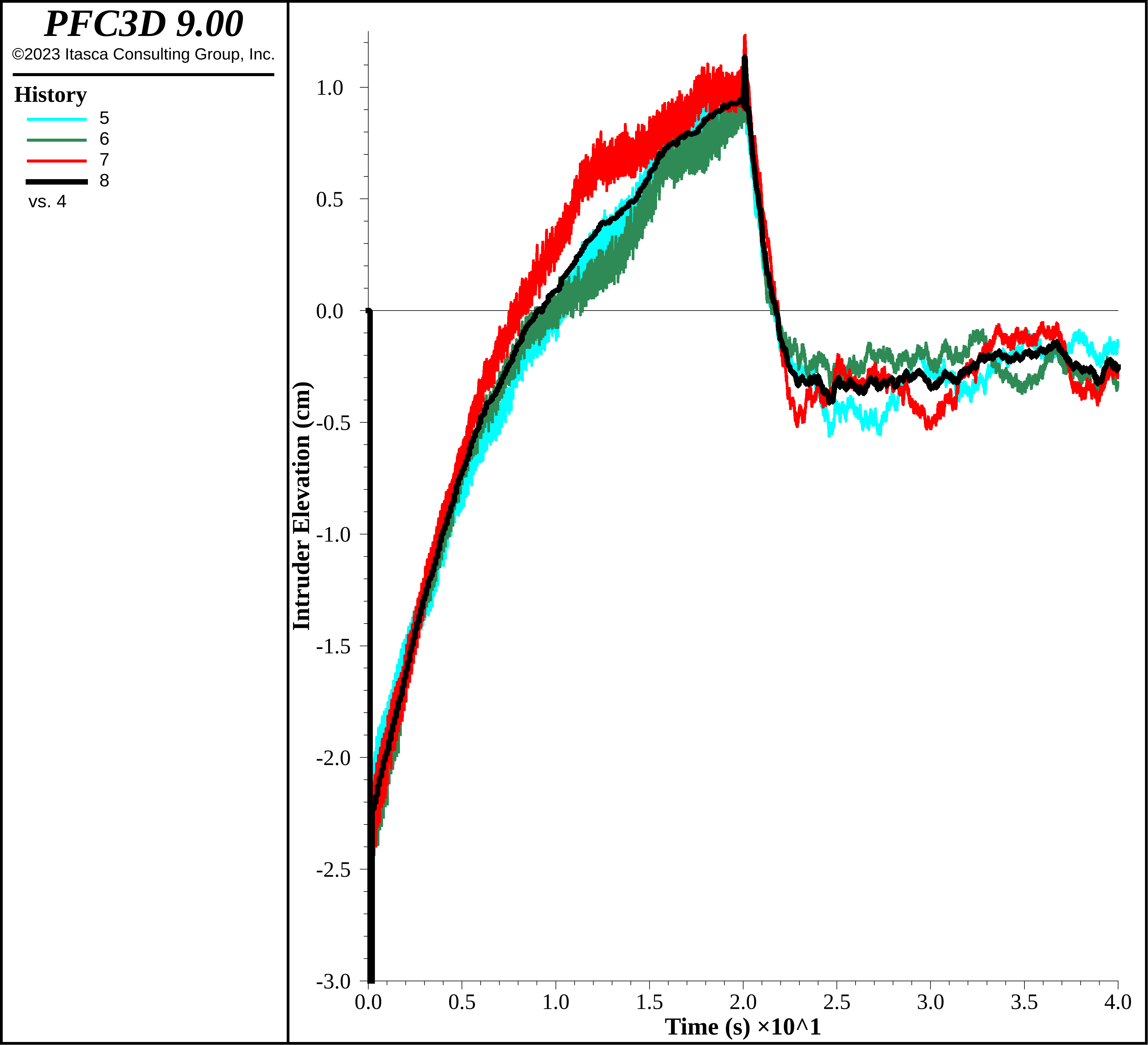
Figure 17: Intruder elevation in the fluidized regime using 100 Hz / 120 cm/s shaking.
The small balls that were originally at the top of the model, along with the intruders, are shown after the additional 20 s of high-frequency shaking. As can be seen, many have migrated back to the top of the model, though some remain trapped below the intruders.
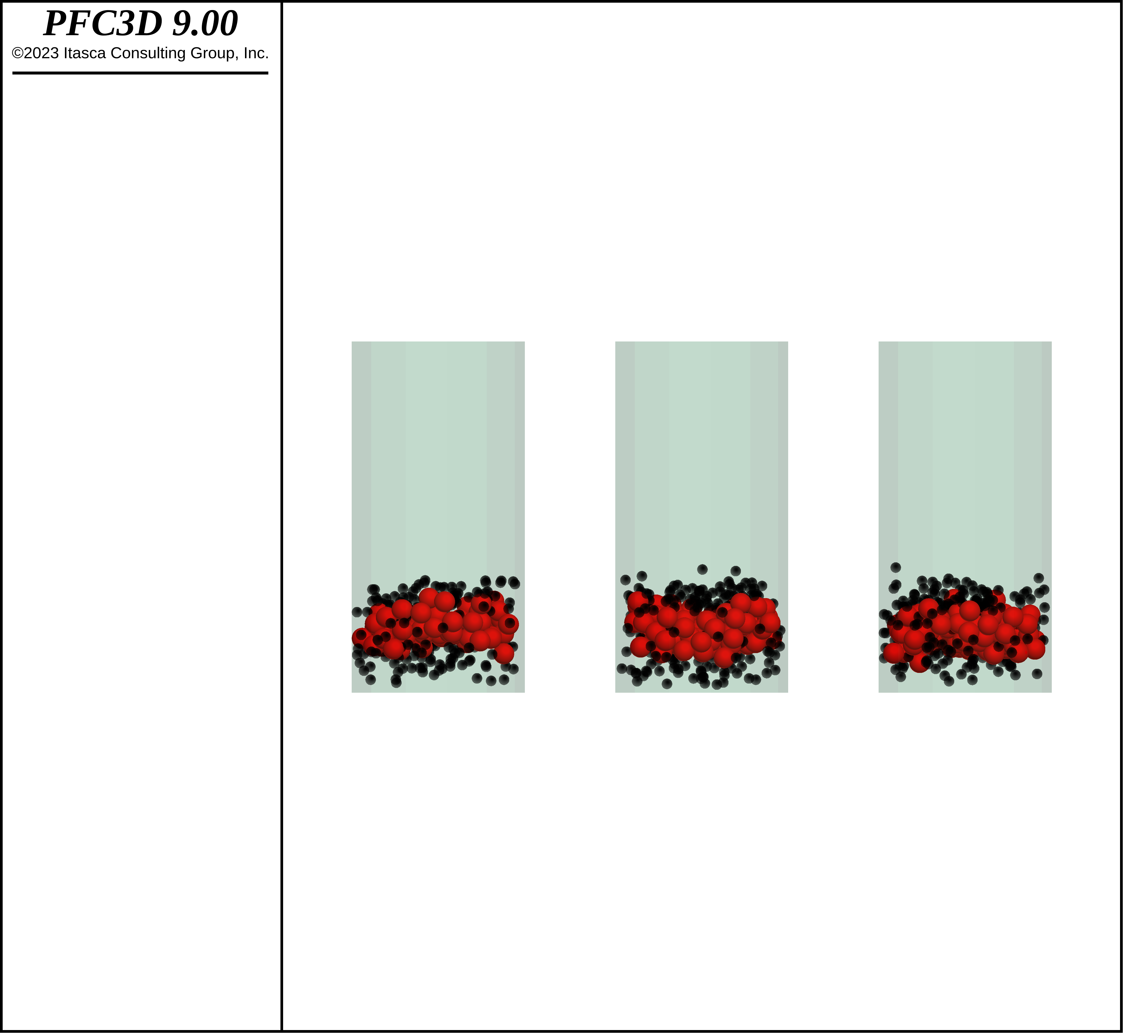
Figure 18: Intruders and top layer of small balls at time 40 s, or after 20 s of additional high-frequency shaking.
Fixing the Timestep
As suggested in the simulations above, fixing the timestep up to 2e-5 s should result in a robust system response with a lower run time. The intruder elevation is shown below fixing the timestep to this value. The run time drops substantially from 5370 s to 3010 s, as one might expect from the results of the smaller models above. The intruder elevation is largely unchanged, even with this much larger timestep. No obvious signs of instability are observed.
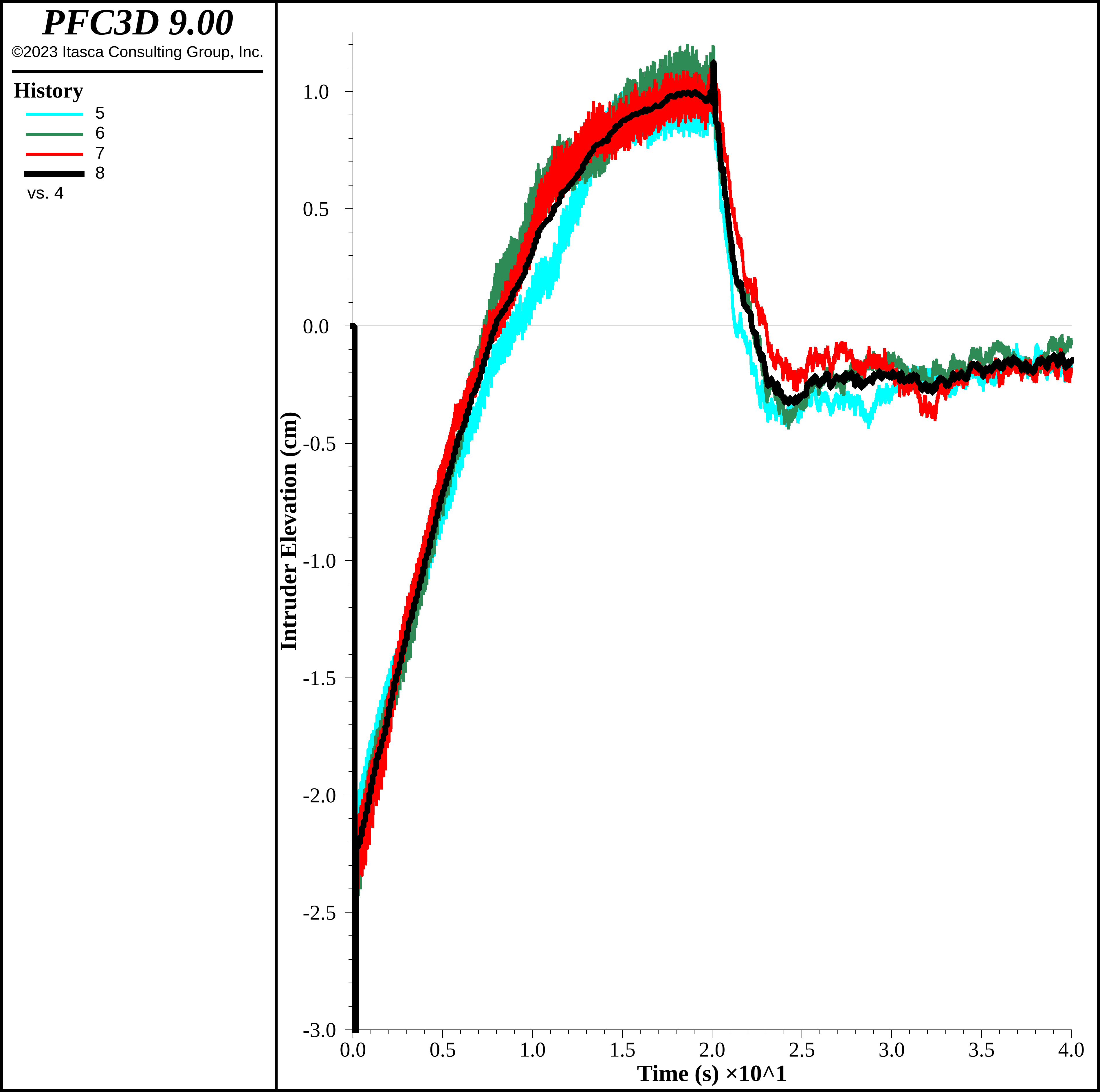
Figure 19: Intruder elevation with timestep fixed to 2e-5 s.
Cell Space Remapping and Contact Creation When Overlapping
Are there additional ways to decrease the computational time? As described in this section of the documentation, pieces (i.e., balls, wall facets, clump pebbles, rigid blocks) are mapped into cell spaces via axis-aligned bounding boxes termed extents. The cell spaces provide an efficient method to find pieces that are in proximity to one another. These extents are used ultimately to create/delete contacts between the pieces, as outlined in the following section. That logic is used to ensure that contacts are created prior to the timestep that the piece surfaces overlap, with remapping in the cell space and contact updating triggered automatically depending on the piece displacement and tolerance extent. The contact remap-interval interval command can be used instead to override this behavior, with cell space remapping occurring at a fixed number of cycles. As it is possible that a contact may be created after overlap, it is essential to use the incremental normal force mode in the contact model whenever modifying the default contact detection strategy.
How does changing the cell space remapping interval impact the model response and running time? The figure below shows the intruder elevation for the entire length of simulation when the remapping interval is set to 10 cycles. As one can readily observe, the model response is clearly within the bounds of the dispersion in realization response, though the simulation time decreases from 5370 s to 3340 s. The rate of cell space remapping appropriate for any given model, and the amount of speed increase, depends on the specific simulation. For highly dynamic problems, it is not uncommon for modifying the remapping interval to result in close to a factor of 2 reduction in computational time. As with the stiffness experiments above, it is often best to run a set of limited models to verify that the model response is robust when changing contact detection behavior.
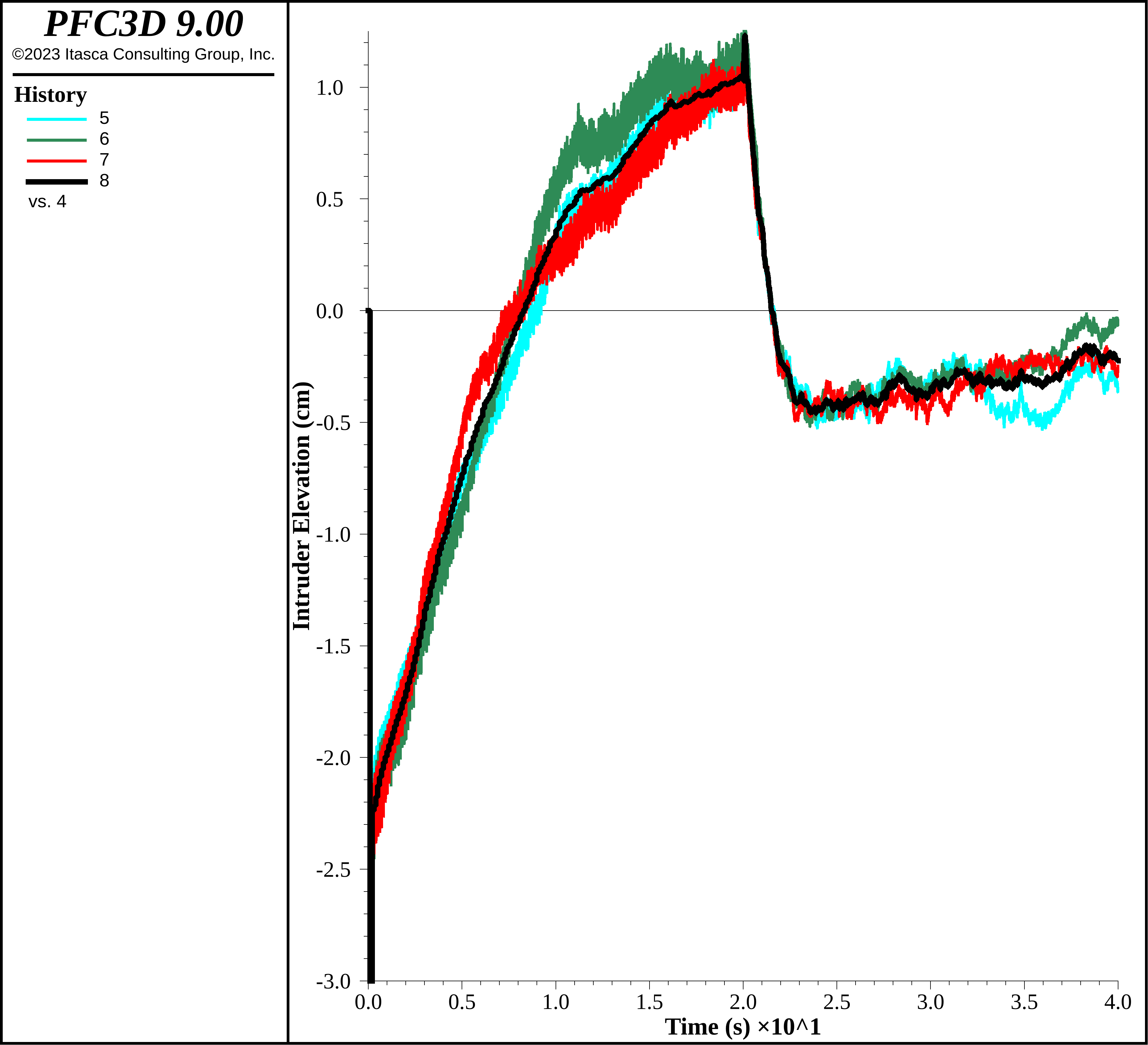
Figure 20: Intruder elevation using a cell space remapping interval of 10 cycles.
Below shows the intruder elevation combining fixing the timestep and setting the cell space remapping interval to 10 cycles. Amazingly, the run time drops from 5370 s to 1750 s, or factor of 3 reduction in run time. This is a substantial decrease in run time without substantial perturbation in model response.
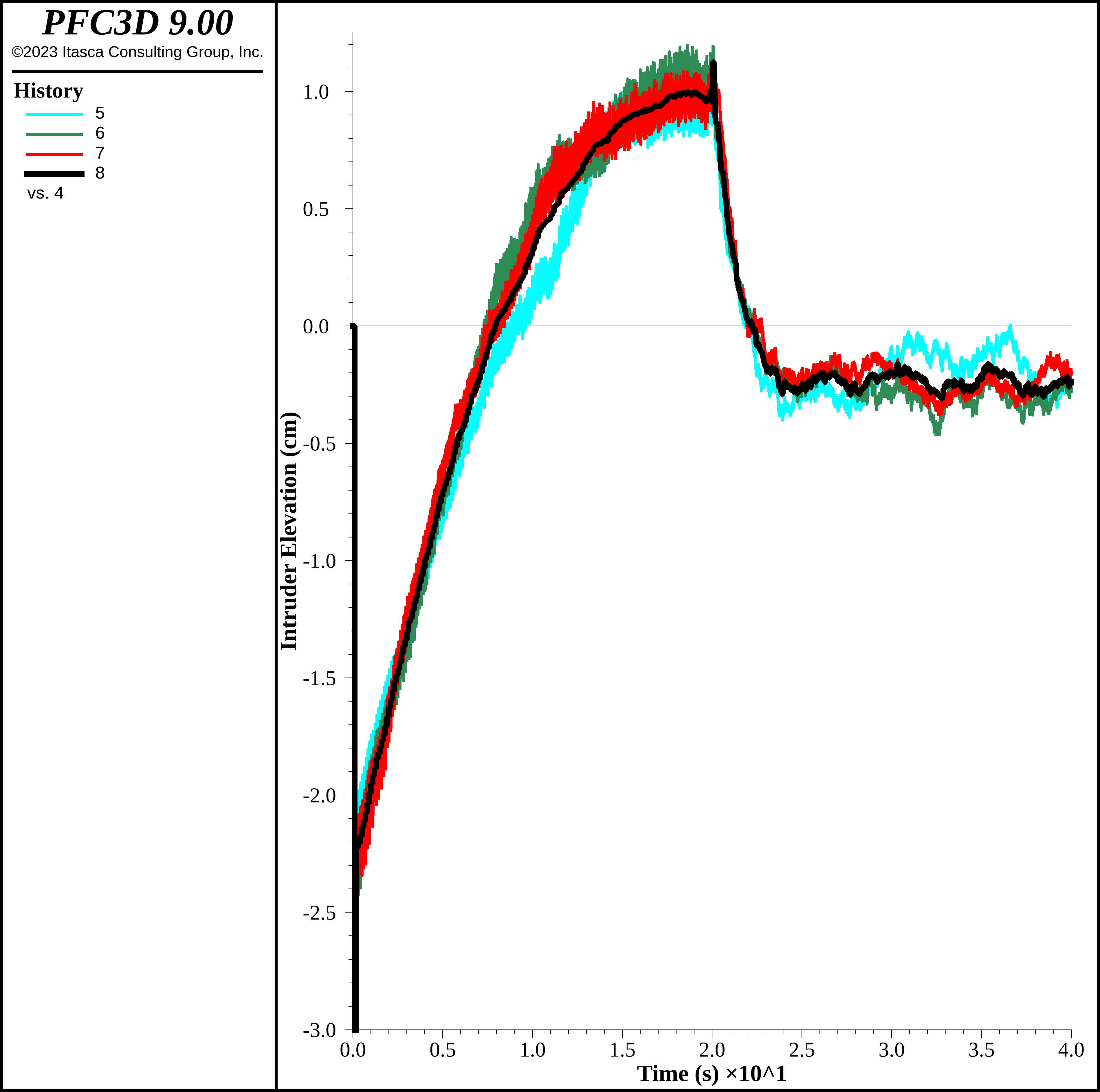
Figure 21: Intruder elevation using a cell space remapping interval of 10 cycles and fixing the timestep to 2e-5 s.
The contact create-on-overlap command, on the other hand, provides one the ability to not create contacts until the pieces actually overlap, greatly reducing the number of contacts. As the computational time is directly proportional to the number of contacts, this can also greatly improve performance. The figure below shows the intruder elevation with this setting enabled. Though the computational time drops from 5370 s to 2690 s, a more substantial drop compared with changing the remapping interval, the rate of intruder elevation increase is faster than the cases above, though the same physical mechanism of small balls moving down along the VCBs is observed. This is similar to the case with the lowest stiffnesses, suggesting perhaps that this effect may be due to the timestep, as both active contacts and contacts that may become active are used to determine the current timestep. Depending on the simulation requirements, this may or may not be of critical importance. In fact, for less dynamic granular flows, changing this contact creation setting may have a negligible impact on model response, but may decrease the computational time by more than a factor of 2.
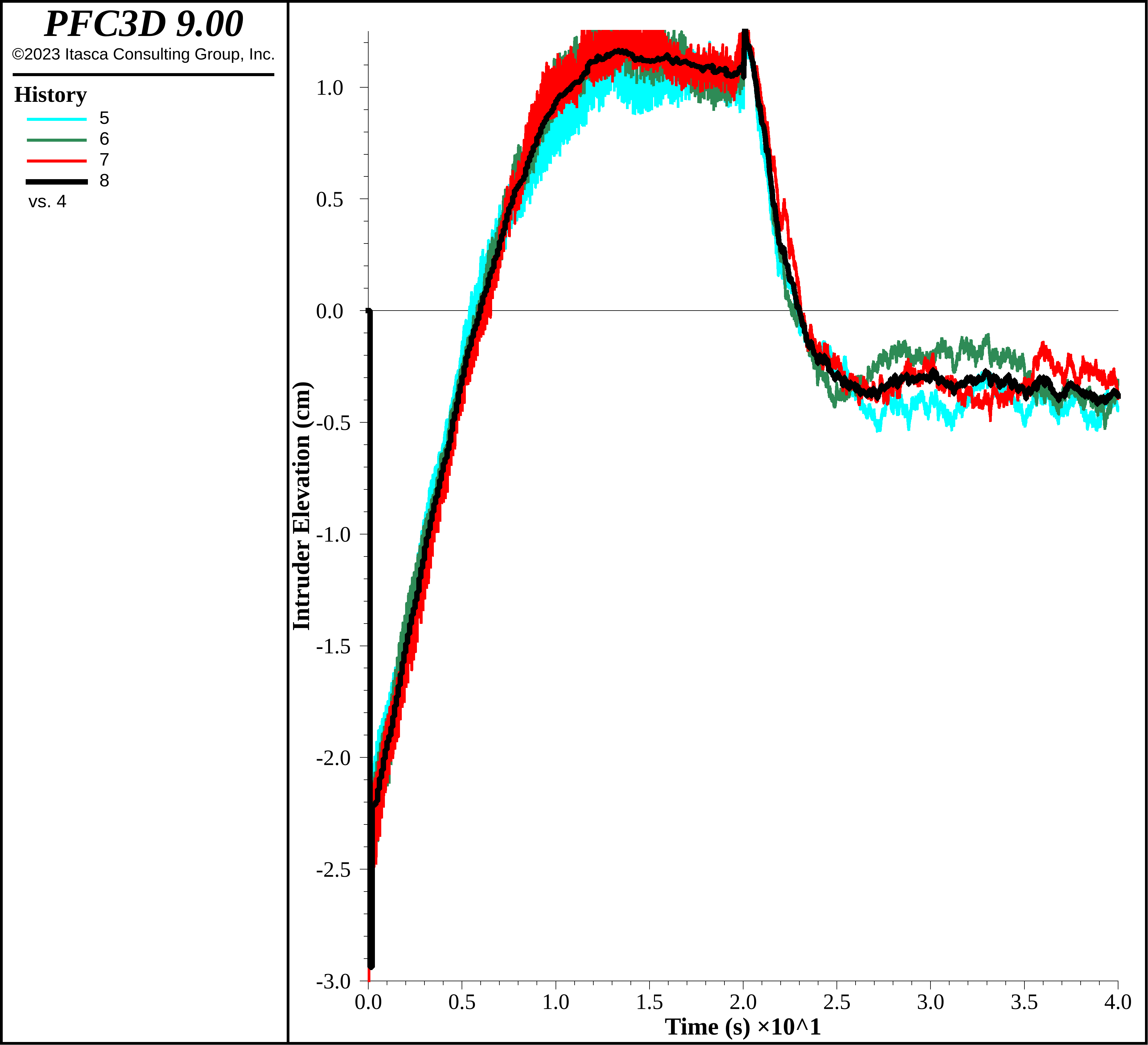
Figure 22: Intruder elevation using the contact create-on-overlap command.
How fast can the simulation go? One can fix the timestep, set the remap interval and the creation-on-overlap setting simultaneously. In some circumstances this may be prudent. The computational time drops to 1030 s, more than a factor of 5 times faster than the original simulation. The results are shown below.
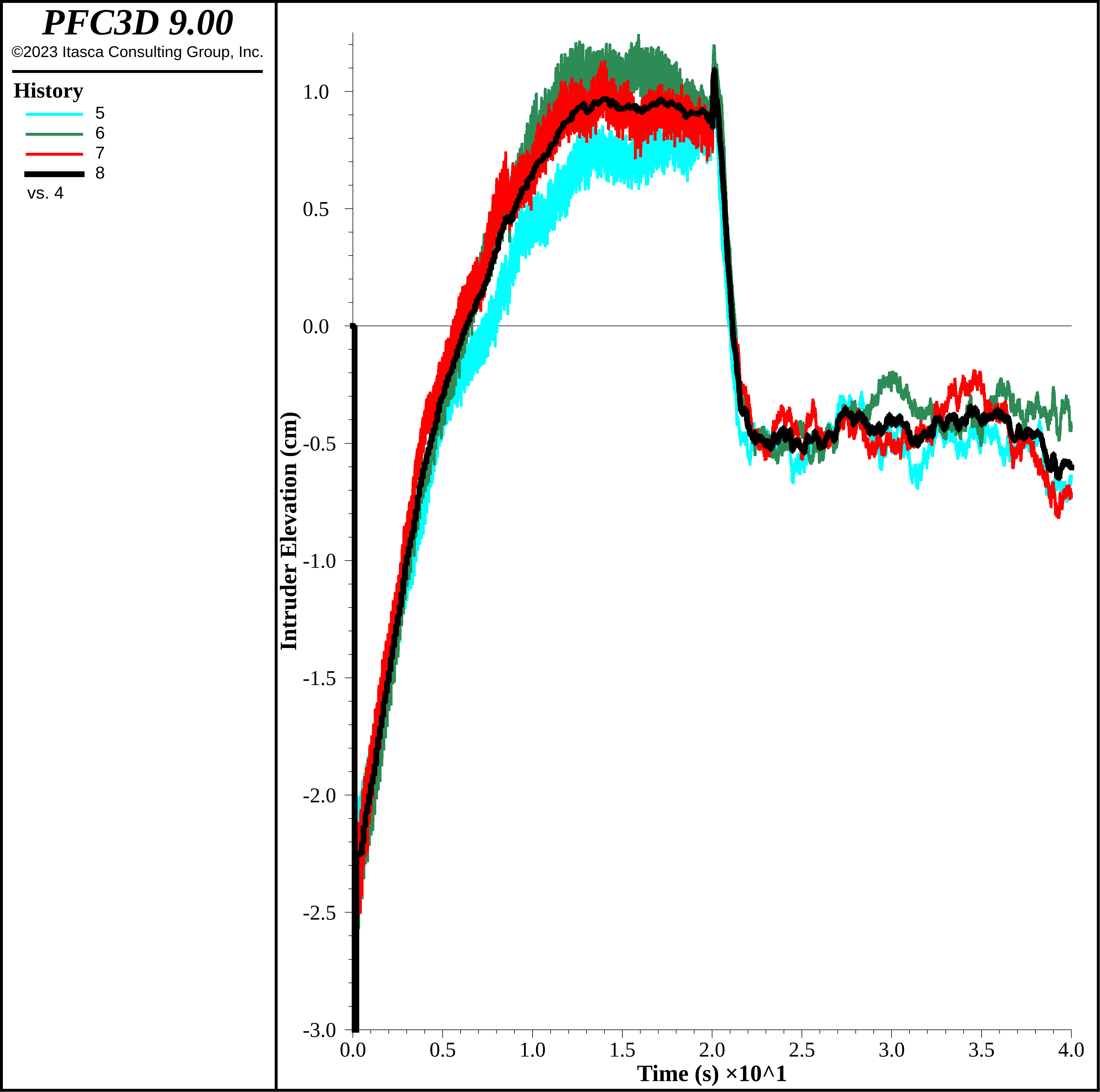
Figure 23: Intruder elevation using a cell space remapping interval of 10 cycles, fixing the timestep to 2e-5 s and the contact create-on-overlap command.
Discussion
This example demonstrates the ability of PFC to model the BNE and RBNE. In detail, convective flow of small particles near VCBs with friction contributes substantially to the BNE. High-frequency shaking changes the nature of the material response to fluidize the specimen, resulting in the RBNE. These simulations are carried out along with discussions of particle upscaling, stiffness scaling, fixing the timestep and relaxing contact detection constraints. Stiffness scaling may result in an order of magnitude decrease in the run time. Fixing the timestep can reduce the run time further. Changing contact detection constraints may decrease the run time as well. Specifically, the model response is relative unperturbed by fixing the timestep and changing the cell space remapping interval in combination, decreasing the run time by a factor of 3. In certain circumstances, one might also only create contacts when the the pieces actually overlap, though the model response is perturbed, perhaps unacceptably, in this very dynamic case. If all three methods are used simultaneously, the run time decreases from the default settings by a factor of 5. This example demonstrates a number of useful strategies that can be used to successfully speed up granular flow simulations.
References
Breu, A.P.J, Ensner, H.-M., Kruelle, C.A., and I. Rehberg, “Reversing the Brazil-Nut Effect: Competition between Percolation and Condensation,” Phys. Rev. Let., 90(1):014302 (2003).
Brown, R.L., “The Fundamental Principles of Segregation,” J. Inst. Fuel, 13:15-19, 1939.
Coetzee, C., “Calibration of the Discrete Element Method: Strategies for Spherical and Non-spherical Particles,” Powder Tech., 364:851-878 (2020).
Hong, D.C., Quinn, P.V. and S. Luding, “Reverse Brazil Nut Problem: Competition between Percolation and Condensation,” Phys. Rev. Let., 86: 3423–3426 (2001).
Kudrolli, A., “Size Separation in Vibrated Granular Matter,” Rep. Prog. Phys, 67(3): 209-247 (2004).
Lommen, S., Mohajeri, M., Lodewijks, G., and D. Schott, “DEM Particle Upscaling for Largescale Bulk Handling Equipment and Material Interaction,” Powder Tech., 352:273–282 (2019).
Rosato, A., Strandburg, K.J., Prinz, F., and R.H. Swendson, “Why the Brazil Nuts Are on Top: Size Segregation of Particulate Matter by Shaking,” Phys. Rev. Lett., 58(10):1038-1040 (1987).
Yan, Z., Wilkinson, S.K., Stitt, E.H., and M. Marigo, “Discrete Element Modeling (DEM) Input Parameters: Understanding Their Impact on Model Predictions using Statistical Analysis,” Comput. Part. Mech., 2:283-299 (2015).
Data Files
MakeModels.dat
; Create a new model with domain 50 cm across. Model units
; are in meters, while the documentation quotes centimeters.
model new
model domain extent -0.25 0.25
; Set to large strain and install gravity.
model large-strain on
model gravity 0 0 -9.8
; Plot every 100000 cycles so the plotting doesn't impact timing.
; This may be necessary as the models are so small.
model update-interval 100000
; Create the container - 10 cm diameter cylinder. The one-wall
; keyword is required for the the range element below.
wall generate cylinder base -0.15 0 -0.1 radius 0.05 height 0.2 ...
    resolution 0.5 one-wall
wall generate cylinder base 0 0 -0.1 radius 0.05 height 0.2 ...
    resolution 0.5 one-wall
wall generate cylinder base 0.15 0 -0.1 radius 0.05 height 0.2 ...
    resolution 0.5 one-wall
; Create a FISH range so that balls clearly fall inside the
; container.
fish define myRange(pos,b)
    loop foreach local w wall.list
        local inside = wall.inside(w,pos)
        myRange = inside
        if inside
            local wf = wall.facet.near(pos)
            local v1 = wall.vertex.pos(wall.facet.vertex(wf,1))
            local v2 = wall.vertex.pos(wall.facet.vertex(wf,2))
            local v3 = wall.vertex.pos(wall.facet.vertex(wf,3))
            local cp = math.closest.triangle.point(v1,v2,v3,pos)
            if math.mag(cp-pos) < ball.rad(b)
                myRange = false
            endif
            exit loop
        endif
    endloop
end

; Set the random seed so that ball generation always results
; on the same packing.
model random 10001
; Generate non-overlapping small balls with diameter 0.6 cm.
ball generate radius 0.003 number [int(1e5)] tries 1000000 ...
    box -0.25 0.25 -0.05 0.05 -0.07 -0.01 ...
    range fish myRange
; Generate non-overlapping large balls, or intruders, with
; diameter 1.2 cm below the small balls.
ball generate radius 0.006 number [int(1e5)] tries 1000000 ...
    box -0.25 0.25 -0.05 0.05 -0.1 -0.07 ...
    range fish myRange
; Assign groups to small and large balls in each cylinder (i.e., per
; realization).
ball group 'small1' range position-x -0.2 -0.1   position-z -0.07 1
ball group 'small2' range position-x -0.05 0.05  position-z -0.07 1
ball group 'small3' range position-x 0.1 0.2     position-z -0.07 1
ball group 'large1' range position-x -0.2 -0.1   position-z -1 -0.07
ball group 'large2' range position-x -0.05 0.05  position-z -1 -0.07
ball group 'large3' range position-x 0.1 0.2     position-z -1 -0.07
; Assign groups to all small and large balls.
ball group 'small' slot 'size' range position-z -0.07 1
ball group 'large' slot 'size' range position-z -1 -0.07
; Assign layer groups for later analysis
ball group '1' slot 'layer' range position-z -0.02 -0.01
ball group '2' slot 'layer' range position-z -0.03 -0.02
ball group '3' slot 'layer' range position-z -0.04 -0.03
ball group '4' slot 'layer' range position-z -0.05 -0.04
ball group '5' slot 'layer' range position-z -0.06 -0.05
ball group '6' slot 'layer' range position-z -0.07 -0.06
ball group '7' slot 'layer' range position-z -0.085 -0.07
ball group '8' slot 'layer' range position-z -0.1 -0.085

; Assign the desired densities, with the intruders being more
; dense than the small balls.
ball attribute density 1500 range group 'small'
ball attribute density 2500 range group 'large'

; Save the initial Brazil nut configuration (BNE).
model save 'BNEIni'
CalibrateStiffness.dat
; Required input:
;   kn      - normal and shear stiffness
;   freq    - frequency of shaking
;   amp     - amplitude of shaking
;   outName - name for tables and save files

; Set CMAT for all contacts.
; *********************IMPORTANT**********************
; The lin_mode must be 1 if changing the contact
; detection or cell space remapping parameters! It
; is also advisable that lin_mode = 1 when fixing the
; timestep.
; *********************IMPORTANT**********************
contact cmat default model linear property kn [kn] ks [kn] ...
    lin_mode 1 fric 0.6 dp_nratio 0.02 dp_sratio 0.02 dp_mode 3

; Apply the CMAT as in case contacts are created before now.
; *********************IMPORTANT**********************
; If changing the timestep computation mode, make sure
; to apply the CMAT if pieces existed before now.
; Fixing the timestep or setting it to be scaled automatically
; creates contacts, even if the CMAT has yet to be specified.
; *********************IMPORTANT**********************
contact cmat apply
; For keeping histories of number of contacts and the average
; position of the large particles.
[large1 = ball.group.list('large1')]
[large2 = ball.group.list('large2')]
[large3 = ball.group.list('large3')]
[small1 = ball.group.list('small1')]
[small2 = ball.group.list('small2')]
[small3 = ball.group.list('small3')]
[elevation = 0]
[nutCnt = 0]
[tmpAvg = 0]
; FISH to compute the history values desired.
fish define contactCount
    contactCount = contact.num
    allContactCount = contact.num.all
    timestep = mech.timestep
    totalTime = mech.time.total
    ; Compute the intruder elevation for realization 1
    elevation1 = (list.sum(ball.pos(::large1)->z)/list.size(large1) - ...
        list.sum(ball.pos(::small1)->z)/list.size(small1))*100
    ; Compute the intruder elevation for realization 2
    elevation2 = (list.sum(ball.pos(::large2)->z)/list.size(large2) - ...
        list.sum(ball.pos(::small2)->z)/list.size(small2))*100
    ; Compute the intruder elevation for realization 3
    elevation3 = (list.sum(ball.pos(::large3)->z)/list.size(large3) - ...
        list.sum(ball.pos(::small3)->z)/list.size(small3))*100
    ; Used to periodically update the average elevation for all
    ; realizations.
    nutCnt += 3
    tmpAvg += elevation1 + elevation2 + elevation3
end
; Define the histories
fish history contactCount
fish history allContactCount
fish history timestep
fish history totalTime
fish history elevation1
fish history elevation2
fish history elevation3
fish history elevation
; Make the velocity time history for shaking, depending on the
; freq and amp parameters.
fish define makeVelocity
    table.delete('vel')
    vtab = table.create('vel')
    local period = 1/freq
    local dt = period/2/100
    local tt = 0.0
    local tt2 = 0.0
    local dt2 = 1/200
    loop while tt < period/4.
        table.value(vtab,table.size(vtab)+1) = vector(tt,amp/(1+math.exp(-130*(tt2-0.055))))
        tt += dt
        tt2 += dt2
    endloop
    table.value(vtab,1) = vector(0,0)
    tt2 = table.size(vtab)
    loop while tt2 > 0
        table.value(vtab,table.size(vtab)+1) = vector(tt,table.y(vtab,tt2))
        tt += dt
        tt2 -= 1
    endloop
    table.value(vtab,table.size(vtab)+1) = vector(tt,0)
    tt2 = table.size(vtab)
    loop while tt2 > 0
        table.value(vtab,table.size(vtab)+1) = vector(tt,-1*table.y(vtab,tt2))
        tt += dt
        tt2 -= 1
    endloop
    ; Current time and period for interpolating the shaking time history.
    freqTime = mech.time.total
    cycleTime = 1/freq
end
[makeVelocity]
; Function to compute the velocity via interpolation of the table.
fish define wallMotion
    if mech.time.total - freqTime > cycleTime
        freqTime += cycleTime
    endif
    local wave = table(vtab,mech.time.total - freqTime) ;...
      ;math.sin(2.0*math.pi*freq*(mech.time.total-freqTime)) * amp
    wall.vel.z(::wall.list) = wave
end
; Call this FISH function every timestep.
fish callback add wallMotion -1
; Function to compute the average intruder elevation
; every period of shaking.
fish define doAverage
    elevation = tmpAvg / nutCnt
    tmpAvg = 0
    nutCnt = 0
end
fish callback add doAverage -1 interval-time [1/freq]
; Simulate for 2 seconds, recording the run time as well.
[timeTot = time.clock]
model solve time-total 2
[timeTot = (time.clock-timeTot)/100]
; Export the intruder elevation history to a table.
history export 8 vs 4 table [outName]
; Export the table to a file. Make sure to use the
; truncate keyword if the file should be overwritten.
table [outName] export [outName+'.tab'] truncate
RunCalibrateStiffness.dat
; Restore the initial model composed of balls and walls.
model restore 'BNEIni'

; FISH function to make a string name depending on an input string
; name (name) and stiffness (inKn).
fish define makeName(name,inKn)
    local outName = name + "KN_" + string(inKn,1,'',1,'e')
    makeName = outName
end

; Run the three realizations with input string name
; (name) and stiffness (inKn).
fish define runModel(name,inKn)
    ; Required input for BNE.dat
    freq = 10
    amp = 0.35
    outName = makeName(name,inKn)
    kn = inKn
    command
        ; Call the data file to set up the run.
        program call 'CalibrateStiffness'
        ; Save the output.
        model save [outName + '.sav']
    endcommand
end

; Remove balls for this smaller model to investigate the
; stiffness impact.
ball delete range position-z -0.04 1
ball delete range position-z -1 -0.08
; Set the plotting update interval to a long time so it doesn't
; influence any timing
model update-interval 100000
; Save the model state so that different simulations can be easily run.
model save 'CalibIni'

; Run tests with stiffnesses ranging from 1e3 to 1e7.
model restore 'CalibIni'
[runModel('CalibD',1e3)]

model restore 'CalibIni'
[runModel('CalibD',5e3)]

model restore 'CalibIni'
[runModel('CalibD',1e4)]

model restore 'CalibIni'
[runModel('CalibD',5e4)]

model restore 'CalibIni'
[runModel('CalibD',1e5)]

model restore 'CalibIni'
[runModel('CalibD',5e5)]

model restore 'CalibIni'
[runModel('CalibD',1e6)]

model restore 'CalibIni'
[runModel('CalibD',5e6)]

model restore 'CalibIni'
[runModel('CalibD',1e7)]

; For the timestep analysis
model restore 'CalibIni'
model mechanical timestep fix 8e-6
[runModel('CalibDTS1',1e5)]

model restore 'CalibIni'
model mechanical timestep fix 1e-5
[runModel('CalibDTS2',1e5)]

model restore 'CalibIni'
model mechanical timestep fix 1.2e-5
[runModel('CalibDTS3',1e5)]

model restore 'CalibIni'
model mechanical timestep fix 1.4e-5
[runModel('CalibDTS4',1e5)]

model restore 'CalibIni'
model mechanical timestep safety-factor 0.9
[runModel('CalibDTS5',1e5)]

model restore 'CalibIni'
model mechanical timestep safety-factor 1.0
[runModel('CalibDTS6',1e5)]

model restore 'CalibIni'
model mechanical timestep fix 2e-5
[runModel('CalibDTS7',1e5)]

model restore 'CalibIni'
model mechanical timestep fix 3e-5
[runModel('CalibDTS8',1e5)]

; Delete the last table
table [makeName('CalibDTS8',1e5)] delete
; Load each table for comparative purposes.
table [makeName('CalibD',1e3)] import [makeName('CalibD',1e3)+'.tab']
table [makeName('CalibD',5e3)] import [makeName('CalibD',5e3)+'.tab']
table [makeName('CalibD',1e4)] import [makeName('CalibD',1e4)+'.tab']
table [makeName('CalibD',5e4)] import [makeName('CalibD',5e4)+'.tab']
table [makeName('CalibD',1e5)] import [makeName('CalibD',1e5)+'.tab']
table [makeName('CalibD',5e5)] import [makeName('CalibD',5e5)+'.tab']
table [makeName('CalibD',1e6)] import [makeName('CalibD',1e6)+'.tab']
table [makeName('CalibD',5e6)] import [makeName('CalibD',5e6)+'.tab']
table [makeName('CalibD',1e7)] import [makeName('CalibD',1e7)+'.tab']
table [makeName('CalibDTS1',1e5)] import [makeName('CalibDTS1',1e5)+'.tab']
table [makeName('CalibDTS2',1e5)] import [makeName('CalibDTS2',1e5)+'.tab']
table [makeName('CalibDTS3',1e5)] import [makeName('CalibDTS3',1e5)+'.tab']
table [makeName('CalibDTS4',1e5)] import [makeName('CalibDTS4',1e5)+'.tab']
table [makeName('CalibDTS5',1e5)] import [makeName('CalibDTS5',1e5)+'.tab']
table [makeName('CalibDTS6',1e5)] import [makeName('CalibDTS6',1e5)+'.tab']
table [makeName('CalibDTS7',1e5)] import [makeName('CalibDTS7',1e5)+'.tab']
table [makeName('CalibDTS8',1e5)] import [makeName('CalibDTS8',1e5)+'.tab']
BNE.dat
; Required input:
;   kn      - normal and shear stiffness
;   freq    - frequency of shaking
;   amp     - amplitude of shaking
;   outName - name for tables and save files

; Set CMAT for all contacts.
; *********************IMPORTANT**********************
; The lin_mode must be 1 if changing the contact
; detection or cell space remapping parameters! It
; is also advisable that lin_mode = 1 when fixing the
; timestep.
; *********************IMPORTANT**********************
contact cmat default model linear property kn [kn] ks [kn] ...
    lin_mode 1 fric 0.6 dp_nratio 0.02 dp_sratio 0.02 dp_mode 3

; Apply the CMAT as in case contacts are created before now.
; *********************IMPORTANT**********************
; If changing the timestep computation mode, make sure
; to apply the CMAT if pieces existed before now.
; Fixing the timestep or setting it to be scaled automatically
; creates contacts, even if the CMAT has yet to be specified.
; *********************IMPORTANT**********************
contact cmat apply
; For keeping histories of number of contacts and the average
; position of the large particles.
[large1 = ball.group.list('large1')]
[large2 = ball.group.list('large2')]
[large3 = ball.group.list('large3')]
[small1 = ball.group.list('small1')]
[small2 = ball.group.list('small2')]
[small3 = ball.group.list('small3')]
[etime1 = 0]
[etime2 = 0]
[etime3 = 0]
[elevation = 0]
[nutCnt = 0]
[tmpAvg = 0]
; FISH to compute the history values desired.
fish define contactCount
    contactCount = contact.num
    allContactCount = contact.num.all
    timestep = mech.timestep
    totalTime = mech.time.total
    ; Compute the intruder elevation for realization 1
    elevation1 = (list.sum(ball.pos(::large1)->z)/list.size(large1) - ...
        list.sum(ball.pos(::small1)->z)/list.size(small1))*100
    if etime1 == 0
        if elevation1 > 0
            etime1 = mech.time.total
        endif
    endif
    ; Compute the intruder elevation for realization 2
    elevation2 = (list.sum(ball.pos(::large2)->z)/list.size(large2) - ...
        list.sum(ball.pos(::small2)->z)/list.size(small2))*100
    if etime2 == 0
        if elevation2 > 0
            etime2 = mech.time.total
        endif
    endif
    ; Compute the intruder elevation for realization 3
    elevation3 = (list.sum(ball.pos(::large3)->z)/list.size(large3) - ...
        list.sum(ball.pos(::small3)->z)/list.size(small3))*100
    if etime3 == 0
        if elevation3 > 0
            etime3 = mech.time.total
        endif
    endif
    ; Used to periodically update the average elevation for all
    ; realizations.
    nutCnt += 3
    tmpAvg += elevation1 + elevation2 + elevation3
end
; Define the histories
fish history contactCount
fish history allContactCount
fish history timestep
fish history totalTime
fish history elevation1
fish history elevation2
fish history elevation3
fish history elevation
; Make the velocity time history for shaking, depending on the
; freq and amp parameters.
fish define makeVelocity
    table.delete('vel')
    vtab = table.create('vel')
    local period = 1/freq
    local dt = period/2/100
    local tt = 0.0
    local tt2 = 0.0
    local dt2 = 1/200
    loop while tt < period/4.
        table.value(vtab,table.size(vtab)+1) = ...
            vector(tt,amp/(1+math.exp(-130*(tt2-0.055))))
        tt += dt
        tt2 += dt2
    endloop
    table.value(vtab,1) = vector(0,0)
    tt2 = table.size(vtab)
    loop while tt2 > 0
        table.value(vtab,table.size(vtab)+1) = ...
            vector(tt,table.y(vtab,tt2))
        tt += dt
        tt2 -= 1
    endloop
    table.value(vtab,table.size(vtab)+1) = vector(tt,0)
    tt2 = table.size(vtab)
    loop while tt2 > 0
        table.value(vtab,table.size(vtab)+1) = ...
            vector(tt,-1*table.y(vtab,tt2))
        tt += dt
        tt2 -= 1
    endloop
    ; Current time and period for interpolating the shaking time history.
    freqTime = mech.time.total
    cycleTime = 1/freq
end
[makeVelocity]
; Function to compute the velocity via interpolation of the table.
fish define wallMotion
    if mech.time.total - freqTime > cycleTime
        freqTime += cycleTime
    endif
    local wave = table(vtab,mech.time.total - freqTime) ;...
    wall.vel.z(::wall.list) = wave
end
; Call this FISH function every timestep.
fish callback add wallMotion -1
; Function to compute the average intruder elevation
; every period of shaking.
fish define doAverage
    elevation = tmpAvg / nutCnt
    tmpAvg = 0
    nutCnt = 0
end
fish callback add doAverage -1 interval-time [1/freq]
; Make a save file,
fish define makeSave
    command
        model save [outName + '_' +string(math.floor(mech.time.total)) + '.sav']
    endcommand
    local minz = list.min(ball.pos(::ball.list)->z)
    local maxz = list.max(ball.pos(::ball.list)->z)
    local diff = (maxz - minz)/8.0
    loop foreach local b ball.list
        local lv = math.floor((maxz - ball.pos(b)->z)/diff)+1
        ball.group(b,'layer2') = string(math.min(lv,8))
    endloop
end
; Add particle traces.
fish define particleTraces
    loop local x(1,3)
        local midx = -0.15 + (x-1)*0.15
        command
            ball trace [vector(midx,0,-0.1)]
            ball trace [vector(midx-0.05,0,-0.1)]
            ball trace [vector(midx+0.05,0,-0.1)]
            ball trace [vector(midx,0,0)]
            ball trace [vector(midx-0.05,0,0)]
            ball trace [vector(midx+0.05,0,0)]
        endcommand
    endloop
end
[particleTraces]
RunBNE.dat
; Restore the initial model composed of balls and walls.
model restore 'BNEIni'

; FISH function to make a string name depending on an input string
; name (name), stiffness (inKn), cell space remapping interval
; (ri) and create-on-overlap behavior (cc).
fish define makeName(name,inKn,ri,cc)
    local outName = name + "KN_" + string(inKn,1,'',1,'e')
    if ri > 0
        outName += "DI_" + string(ri)
    endif
    if cc == true
        outName += "CC"
    endif
    makeName = outName
end

; Run the three realizations with input string name
; (name), stiffness (inKn), cell space remapping interval
; (ri) and create-on-overlap behavior (cc).
fish define runModel(name,inKn,ri,cc)
    ; Required input for BNE.dat
    freq = 10
    amp = 0.35
    outName = makeName(name,inKn,ri,cc)
    kn = inKn
    ; Set the remap interval.
    if ri > 0
        command
            ball remap-interval [ri]
            wall remap-interval [ri]
        endcommand
    endif
    ; Set create-on-overlap behavior.
    if cc
        command
            contact create-on-overlap true
        endcommand
    endif
    command
        ; Call the data file to set up the run for the
        ; convective portion.
        program call 'BNE'
        ; Make save files every 2 seconds.
        fish callback add makeSave -1 interval-time 2
        ; Cycle for 20 seconds and record the run time.
        [timeTot = time.clock]
        model solve time-total 20
        [timeTot = (time.clock-timeTot)/100]
        ; Compute the average entrainment time, or time for the intruders to be
        ; entriely entrained in the small ball bed.
        [eList = list.seq(etime1,etime2,etime3)]
        [eTime = list.sum(eList)/list.size(eList)]
        ; Compute the standard deviation as well
        [stdETime = math.sqrt(list.sum((eList - etime)^2/(list.size(eList)-1)))]
        ; Save the model state.
        model save [outName + 'Convect.sav']
        ; Adjust for the fluidization portion.
        ; Remove the save file FISH function, as done every 2 seconds, and
        ; hook it back up to do every 10 seconds.
        fish callback remove makeSave -1
        fish callback add makeSave -1 interval-time 10
        ; Make a new shaking history for this regime and set pertinent parameters.
        [freq = 100]
        [amp = 1.2]
        [makeVelocity]

        ; Change the average timing as well.
        fish callback remove doAverage -1
        fish callback add doAverage -1 interval-time [1/freq]

        ; Cycle for 20 seconds and record the run time.
        [timeTot2 = time.clock]
        model solve time 20
        [timeTot2 = (time.clock-timeTot2)/100]
        ; Compute the total time for all cycling.
        [timeTot += timeTot2]
        model save [outname + 'Final.sav']
    endcommand
end

; Set the plotting update interval to a long time so it doesn't
; influence any timing
model update-interval 100000
; Save the model state so that different simulations can be easily run.
model save 'BNEIniStart'

; Test 1 - default settings.
model restore 'BNEIniStart'
[runModel('BNE',1e5,0,false)]

; Test 2 - cell space remap interval of 10 cycles.
model restore 'BNEIniStart'
[runModel('BNE',1e5,10,false)]

; Test 3 - create-on-overlap true.
model restore 'BNEIniStart'
[runModel('BNE',1e5,0,true)]

; Test 4 - cell space remap interval of 10 cycles
; and create-on-overlap true.
model restore 'BNEIniStart'
[runModel('BNE',1e5,10,true)]

; Test 5 - default settings except timestep is fixed
; to 2e-5 s.
model restore 'BNEIniStart'
model mechanical timestep fix 2e-5
[runModel('Fix',1e5,0,false)]

; Test 6 - cell space remap interval of 10 cycles and
; timestep is fixed to 2e-5 s.
model restore 'BNEIniStart'
model mechanical timestep fix 2e-5
[runModel('Fix',1e5,0,false)]

; Test 7 - cell space remap interval of 10 cycles,
; create-on-overlap true and timestep fixed to
; 2e-5 s.
model restore 'BNEIniStart'
model mechanical timestep fix 2e-5
[runModel('Fix',1e5,10,true)]
Endnote
| Was this helpful? ... | Itasca Software © 2024, Itasca | Updated: Nov 12, 2025 |
