FLAC2D Modeling • Tutorials
Tutorial: Illustrative Model — Mechanics of Using FLAC2D
This tutorial provides the new user an initial look at the basics of modeling with FLAC2D. The structure of this tutorial, delineated below, corresponds to the general structure for FLAC2D modeling that is presented at length in the topics found in the Problem Solving with FLAC section that is also charted in General Solution Procedure, Illustrated.
This tutorial problem presents a trench excavated in a soil with low cohesion. After failure is observed during excavation, support is added to stabilize the trench.
For this tutorial, the sequence charted in General Solution Procedure, Illustrated may be broken down as follows.
First, a model must be set up in FLAC2D, which comprises the first seven steps below.
Create a project for the model.
The project acts as a central collection of all resources and outputs that will be part of the FLAC2D model.
Create a mesh that discretizes the model volume.
The grid defines the geometry of the problem.
Assign names to regions of the model by using Groups.
Groups are used to label areas of specific interest in the model.
Assign constitutive behavior and material properties.
The constitutive behavior and associated material properties dictate the type of response the model will display upon disturbance (e.g., deformational response due to excavation).
Apply boundary conditions.
Assign initial conditions.
Initial conditions define the in-situ state (i.e., the condition before a change or disturbance in the problem state is introduced).
Step to initial equilibrium state.
After the model setup is complete, the initial equilibrium state is calculated for the model.
Next, the model is ready for alteration, perturbation, or other examination. This is usually the point where the intended analysis really begins. The next steps shown are ones that might be looped or branched in many variations, depending on the needs of the analysis.
Alteration of the model as required by the problem.
Alteration(s) are then made (excavate material, change boundary conditions, install support, etc.), and the resulting response of the model is calculated. At this point, the nature of the problem will determine what steps will follow; there is no specific normative approach. In the case of this tutorial, the following steps conclude the analysis.
Examine model response (plotting).
Further alteration (e.g., install support).
Project completion (storage).
Solutions
The actual solution of the problem is different for an explicit program like FLAC2D than it is for conventional implicit-solution programs. (This is a large topic; see the FLAC Theory and Background section.) FLAC2D uses an explicit time-marching method to solve the discretized equations. The solution is reached after a series of computational steps. In FLAC2D, the number of steps required to reach a solution can be controlled automatically by the code or manually by the user. However, the user ultimately must determine if the number of steps is sufficient to reach convergence to equilibrium. In this tutorial, the way this is done is described in the Step to Equilibrium and Meaning of Equilibrium sections below.
Building a Data File
FLAC2D is a command-driven program. Those commands can be issued from the command prompt, or, in a number of cases, they are generated interactively by the user interface. There is no difference between the commands as issued from one place or the other, merely the matter of efficiency and speed in the issuing, and user preference.
However, there is a third place where commands are saved/recorded: the data file. The data file is essentially a batch file, that is, a list of commands that can be issued and processed in an unbroken sequence. This is both more efficient than either the command prompt or mouse/keyboard commands—either of which is limited to issuance of one command at a time—and has the added advantage of providing a readable representation of a problem from beginning to end.
Model construction in FLAC2D is thus a matter of data file construction. Though typing a data file in its entirety prior to any command processing is possible, in practice this is rarely done. Instead, a final data file is arrived at in a stepwise fashion that is usually a blend of commands from the file itself and/or other data files, the command prompt, and the user interface, not to mention the number of “drafts” that occur in refining the modeling approach taken to best represent the problem. The art of data file construction in FLAC2D is a matter of efficiently using all three command sources, as well as the save/restore system, to work through the problem.
The State Record Pane
In FLAC2D, all operations that modify the current model state do so by issuing a command. Operations that only affect the program or project state do not have this requirement and generally do not issue a command in the interface, although commands exist that only change those states. All commands that occur in a given model state are recorded in the State Record. This record is included in save files that represent the model state created using the model save command. Commands are recorded regardless of whether they are generated directly by the user or interactively by the user interface. These commands are available for review in the State Record tab in the Commands area. This state record may be played back directly using the program playback command, or it may be converted into an equivalent data file for later repetition or parameterization.
The state record does not record the contents of a data file that is executed. These commands are considered to be already recorded in the data file itself. Rather, the record tracks the data file name, size, and last modified stamp for reference.
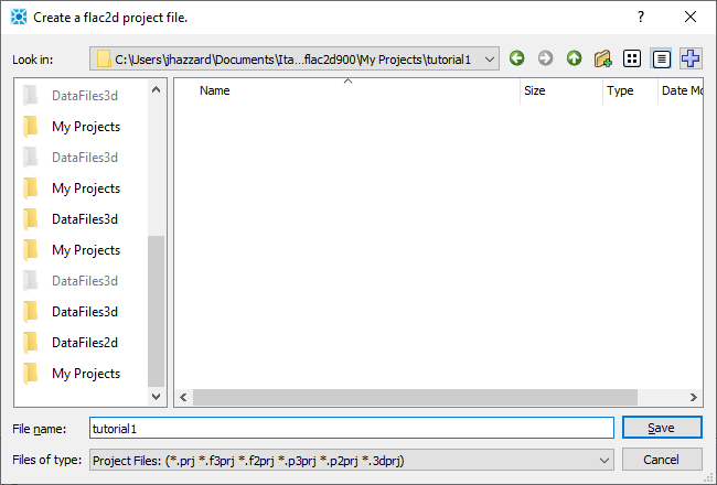
Create a New Project
Create a project for this tutorial.
Choose from the main menu.
Navigate to the folder where the project file will be saved.
Name the project “tutorial1” in the
File Namefield.press or press Enter .
Create a Data File
For this tutorial, a single complete data file for the problem will be created.[1]
Select or press Ctrl + N.
At the
File Namefield, enter “tutorial”.Press or press Enter .
Note the new data file is now shown in the FLAC2D Workspace area.
Discussion
When a project file is created and saved, FLAC2D uses the folder containing that project file as the current working directory. This location will be the default for most file-managing dialogs presented in the user-interface. In addition, any command that saves a file may be issued without a path, as the working directory is assumed if no path is supplied.[2]
Creating a project at the outset of any modeling process is the strongly recommended approach to using FLAC2D. The project handles a range of tasks for managing the modeling project, in addition to the ones described above. The existence of a project makes retaining settings, re-opening or restoring files, and project support and archiving significantly easier.
Refer to the Projects section for complete information on working with projects.
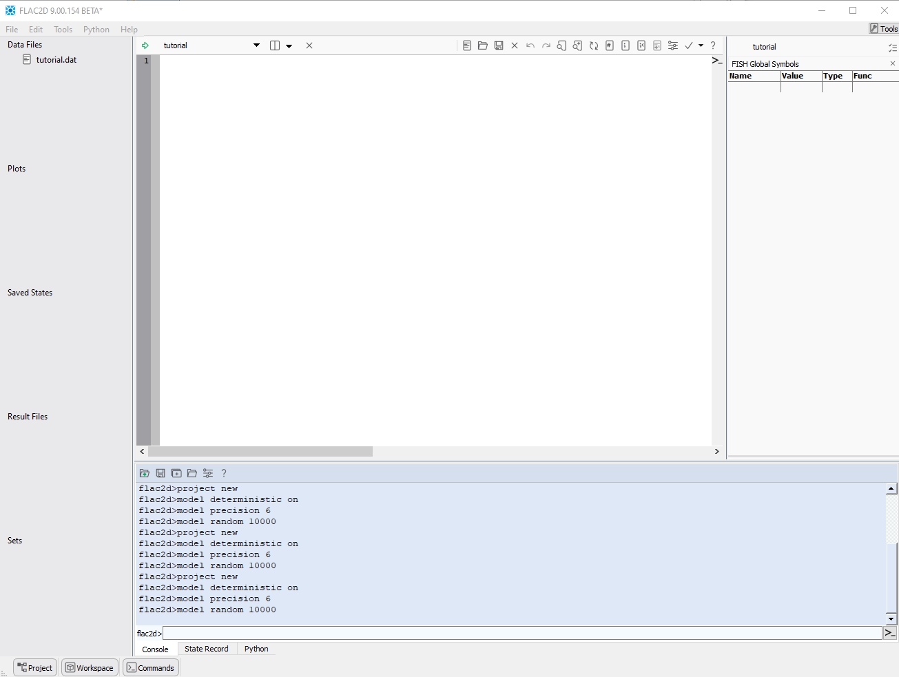
In the Interface
After creating the project and data file, some additional aspects of the program’s behavior may be noted.
Tip
See the topic Layout for a quick review of the nomenclature for the parts of the program layout mentioned here.
The data file has been added to the Project panel on the left.
Also note that when the data file is created, a blank data file is opened in the Workspace.
The name of the data file appears at the top of the Workspace followed by a drop down menu selector that allows the content (data file, or plot, or other item) to be created or changed in the Workspace.
The toolbar (at the top) contains tools for working in the editor. The Tools panel on the right displays editor-specific controls. For any content in the Workspace (data file, plot, sketch set, etc.), the Tools panel and the Workspace toolbar will contextually supply tools/facilities appropriate for the current content.
The Console tab is visible at the bottom in the Commands area. This is where information related to command processing is displayed. Commands may also be typed and executed interactively in the Console.
Visibility of the three principal areas of the program (Project, Workspace, and Commands) can be toggled using the buttons at the bottom left in the program status bar.
Generate the Grid
The grid for this problem is created with one command.
Type the lines below into the “tutorial.dat” data file (or cut and paste them directly from below).
model new

; Create zones
zone create tunnel-quad ...
        point 0 (0,0) point 1 (10,0) point 2 (0,10) ...
        size 3,5,7 ...
        ratio 1,1,1.5 ...
        dimension 1 4 fill group 'exc'

zone reflect normal -1,0
zone reflect normal 0,-1
zone delete range position-y 0 10

model save 'geom'
Press the Execute button (
 ). The commands are processed and echoed in the Console output.
Activate the Model in the Workspace by choosing from the drop-down menu at the top of the Workspace.
Use the mouse wheel to zoom in and out. To pan, hold down the right mouse button, followed by the left mouse button. See View Manipulation for more ways of manipulating the view when examining the model.
Note
Tip
View the data file and the Model pane side by side by clicking on the split icon ![]() at the top and choosing and then choose what to display in each tile from the drop down menu at the top.
at the top and choosing and then choose what to display in each tile from the drop down menu at the top.
Discussion
The first command clears FLAC2D of model-state information (see model new for reference). To keep things simple, the entire data file is re-run using ![]() each time lines are added as this tutorial progresses. Putting
each time lines are added as this tutorial progresses. Putting model new at the start ensures the model will run without error each time this happens.
Note
Comments are denoted with a semi-colon (;) and are ignored by FLAC2D.
The second command creates part of the geometry. In that line, a tunnel-quad primitive is used to create zones. The keywords that follow the name of the primitive specify size, grid spacing (ratio), and brick-size (dimensions). This command occupies five typed lines of text, but through use of the continuation operator ( … ) FLAC2D treats these as one line, making it a single command.
The zone create2d tunnel-quad command creates half of the desired trench in an upside-down orientation (the command assumes creation of a quarter of a rectangular tunnel, but this example manipulates the resulting mesh to form the trench geometry).
To complete the trench and turn it right size up, two reflections are performed (zone reflect) and then the top half is deleted (zone delete).
Creating a problem’s grid with primitives is a fast and efficient method of constructing zones. However, as the complexity of model geometry increases, the use of primitives also gets increasingly difficult, and FLAC2D offers other methods of constructing grids that may be preferable. Using the Sketch pane is described in Tutorial: Quick Start (FLAC2D). A more thorough discussion of zone construction methods and the multiple considerations that go into grid construction are described in Grid Generation in FLAC2D.
It is a recommended practice to save the model state at the point where the zones for the problem geometry are created. Since one zone create command is sufficient to obtain the geometry needed for this problem, the final line above saves the model state in the file “geom.sav” (note the file extension is added automatically).
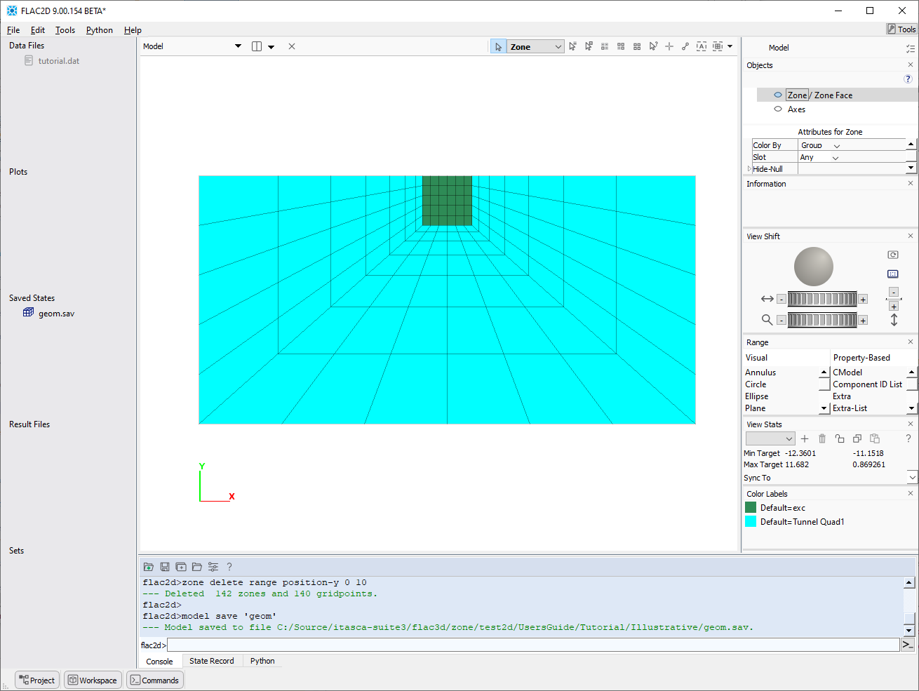
In the Interface
After processing the commands that generate the problem mesh, some aspects of the interface can be observed.
An asterisk (*) appears next to the program name and version in the title bar to indicate the project is not saved. In FLAC2D, when an asterisk appears adjacent to a name in a list or on a title bar, it indicates that the item has been modified since it was last saved.
The “tutorial.dat” file does not have an asterisk next to it. This is because the file was automatically saved when the Execute button (
) was pressed—which is the normal program response when that button is used.The Project panel now shows “geom.sav” in the “Saved States” list.
The Model in the Workspace displays the model zones that are created.
The commands that were processed from the data file when the Execute button (
) was pressed are echoed in the console output. The observant will note that the effect of pressing the button is really to cause a program callcommand to be issued for the currently active data file.
Create Model Groups
Next zone face groups are created that will be used later when setting up boundary and initial conditions (note that zone edges in 2D are termed faces to be consistent with 3D). In addition, the five excavation stages are created by grouping the zones that will be removed from the model at each stage.
Make the Model active, if it isn’t already (choose from the drop-down menu at the top).
Press the Assign group names to faces automatically … button (
 ).
).In the ensuing dialog, check Ignore Existing Group Names and press .
In the lower center tab group, make the State Record active by clicking on its tab.
Select the line
>>zone face skinRight-click and choose Copy as Data File.
Make the tutorial data file active, set the cursor at the end of the file, and paste (Ctrl + V or ).
Create groups for each of the five excavation stages. Type (or copy-paste from below) the lines that create the five groups (“exc1” through “exc5”) in the data file.
At the end of the data file, type (or copy-paste from below)
model save "groups".The commands from this step and step (6) that have been added to “tutorial.dat” should appear as below:
zone face skin

zone group "exc1" range position-x -1 1 position-y -0.8 0
zone group "exc2" range position-x -1 1 position-y -1.6 -0.8
zone group "exc3" range position-x -1 1 position-y -2.4 -1.6
zone group "exc4" range position-x -1 1 position-y -3.2 -2.4
zone group "exc5" range position-x -1 1 position-y -4.0 -3.2

model save 'groups'
Note that these commands could also have been generated interactively using range selection tools in the Model pane. This was not done here for brevity.
Rerun the model to this point by pressing solve (
).
Discussion
The Assign group names to faces in the Model pane is a tool that identifies groups of contiguous zone faces based on a break angle (45° by default) and creates automatically-named zone face groups for them. [3] In this case, using the tool results in four face groups being created, one for each “side” of the problem’s cubic geometry.
Note something specific happens here: the model state is changed to include the newly created face groups. However, the command that caused this change is not a part of the “tutorial” data file. In order to ensure the data file is complete, it is necessary to capture the command that created the groups. The State Record tab facilitates this. As its name implies, the State Record records any command (from a data file, from the command prompt, from the user interface) that changes the model state, as it is issued, and stores it in a record. The record therefore contains all commands necessary to create the current model state. Because the object for this tutorial is to arrive at a single complete data file, the State Record pane is used to copy the command that was used to create the face groups with the Auto Assign Face Groups tool and paste it into the data file.
The zones in each of the five excavation stages are grouped as well using the zone group command. Here one of the principal advantages of putting objects into named groups is clear: the names assigned to groups can have a logical relationship to one another and to the rest of the model. When the commands that will be used to perform the excavation sequence appear later, the names of the groups will help clarify what is going on in the commands.
Once the logical parts of the model have been identified and put into groups, it is a good idea to save the model state (review :ref:-solutionasflac3dproject-). CS: this figure (or something similar) is still a good idea, but gone for now (see flac3d 6 doc set) The final line that is added at step (7) does this.
When to Group
Designating groups is not strictly necessary at this stage, but it is highly advisable, as construction of commands that use groups as range targets is usually faster, easier, and perhaps more innately sensible than constructing a range with the other range elements. Groups are also quite useful later on for plotting. Lastly, using groups helps conceptualize the model in terms of its meaningful parts. That said, the Model pane can be used for model object selection and grouping at any time in a modeling project.
Ranges and Groups, Briefly
As this tutorial provides a first look at the FLAC2D range logic and groups, a word to distinguish them may be of use. A range is composed of one or more selection criteria that identify the objects on which a command should operate—if a range is not supplied on a command, all possible target objects of the command will be affected (see How Commands Work). A group is what its name implies: a collection of specific objects going by a given group name.
The initial definition of a group is made by specifying a range that determines the member objects.
zone group "lower" range position-y 1 100
This creates a group of zones named “lower”. It is possible that after cycling, the zones that fall in that range y 1 100 will be different. The zones in the group “lower”, however, will be the same.
Once created, a group can be the target of a command by specifying it as the defining criterion of a range. Consider:
zone cmodel assign elastic range group "lower"
This assigns the Elastic model to the zones in the group “lower”.
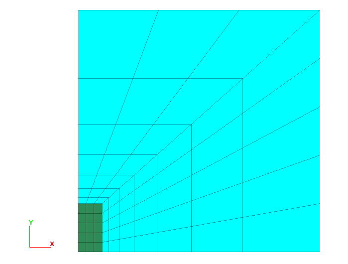
In the Interface
Use the i content selector in the Workspace to make the Model active (if it isn’t already). The model should appear similar to the image below.
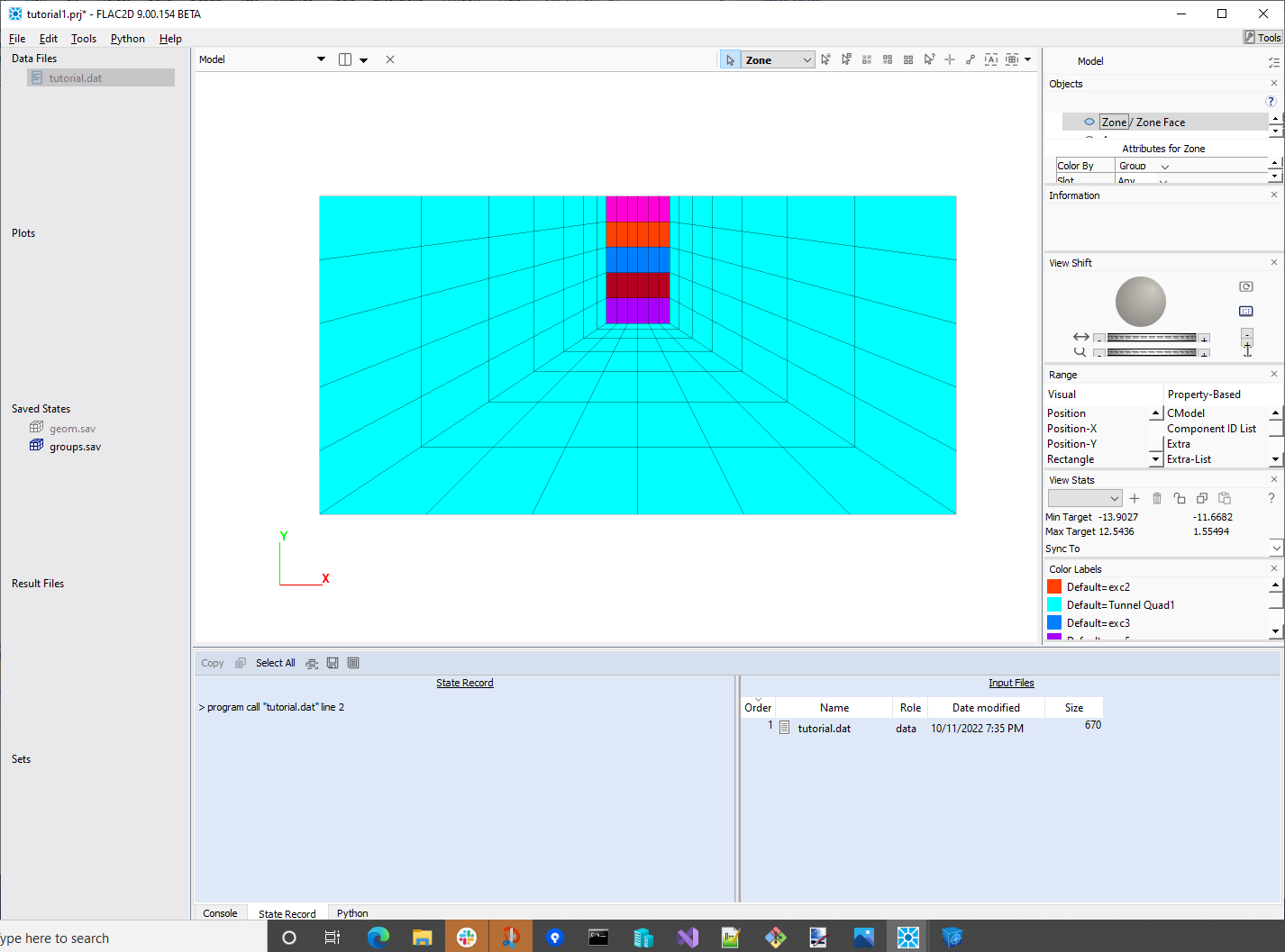
Zones that are created by any method—with the zone create command, or through Sketch, are rendered in the Model pane.
This area is capable of allowing the user to interact with model elements—zones or zone faces at this stage of the process—via mouse-driven selection tools. Any area of the model that may be of specific interest can be selected and defined to be a group.
The “Saved States” section of the Project tile now lists two .sav files. The active model state is “groups.sav” (the inactive model state listed here, “geom.sav”, is grayed out).
The “Objects” control set in the Control Panel indicates what is rendered in the view. At any time, the zones in a model may be rendered as either zones or zone faces, but not both. For this reason, the item is shown as “Zone / Zone Faces”, with a box around the currently rendered item. Clicking the word “Zone” or “Zone Faces” will set the clicked item to be the one rendered in the pane. As an immediate visual feedback, when zones are being rendered, the faces are outlined in black. When Zone Faces are being rendered, the faces are outlined according to their color label (by default, the label is “none” and the color is light blue).
Double-click the item “geom.sav” in the “Saved States” section of the Project tile. Choose Zone Face from the drop-down menu at the top to show the faces (edges in 2D). As “geom.sav” is the active state, all zone faces are rendered in a single color, because there are no face groups in this model state. Double-click “groups.sav” to restore that model state, then click in the Model pane to reactivate it. Now the model is displayed with its excavation groups visible. Check the “Color Labels” control set to identify the color assignments in the current rendering.
To experiment, open the “Rendering” item in “Attributes for Zone Face” and observe the effect of changing the settings it contains.
Rendering in either the Model pane or in a Plot follows the same basic principle, which is also explained in In the Interface following the topic Examine Model: Plotting.
The items to be rendered in the view are listed in the upper section of the “Objects” (Model pane) or “Plot Item List” (for a Plot) control set in the Control Panel.
With an object selected in the upper section, the lower section provides an “Attributes” set that supplies controls for setting how the selected object should be rendered.
Specifying Models, Boundaries, and Initial Conditions
Next a series of commands is added to complete the initial model definition.
Type or copy-paste the lines below into the “tutorial” data file.
; assign constitutive model, initial, and boundary conditions
zone cmodel assign mohr-coulomb
zone property density 1000 young 4.5e8 poisson 0.25 ...
              friction 35 cohesion 1e3 tension 1e3

zone face apply velocity-normal 0 range group "Bottom"

model gravity (0,-10)
zone initialize-stresses ratio 0.5
zone face apply stress-normal 0 ...
  gradient 0,[10*1000*0.5] range group "West" or "East"
Rerun the model to this point by pressing solve (
).
Discussion: Assigning a Constitutive Model
Once the grid generation and model partitioning (grouping) is complete, one or more material models and associated properties must be assigned to all zones in the model. These are done using the commands zone cmodel assign and zone property. Here, the zone cmodel assign command that assigns a mohr-coulomb model is supplied without a range. Consequently, it will be applied to all zones in the model.
Properties are set with zone property commands in a way that spans model assignments. Setting the Young’s modulus property without a range will set it for any zone whose assigned constitutive model uses a young property (and this is most of them). Limiting the specification of a property to zones with a particular constitutive model assignment is done by using a range that invokes the constitutive model assignment as a criterion in a range. For example, contrast the following with what is given above.
zone property young 1e4 range model mohr-coulomb
This command would set the young property only for zones that have been assigned the mohr-coulomb model.
Constitutive Models and Properties
FLAC2D has nineteen built-in mechanical material models (Constitutive Models). Three models are sufficient for most analyses the new user will make: null, elastic, and mohr-coulomb.
The null model represents material that is removed or excavated from a model. The elastic model assigns isotropic elastic material behavior. The mohr-coulomb model assigns Mohr-Coulomb plasticity behavior.
The models elastic and mohr-coulomb require that material properties be assigned via the zone property command. For the elastic model, the required properties are bulk and shear modulus, or Young’s modulus and Poisson’s ratio.
NOTE: Bulk modulus, \(K\), and shear modulus, \(G\), are related to Young’s modulus, \(E\), and Poisson’s ratio, \(ν\), by the following equations:
or
The following are required properties for the Mohr-Coulomb plasticity model:
bulk and shear moduli, or Young’s modulus and Poisson’s ratio;
friction and dilation angles;
cohesion; and
tensile strength.
If any of these properties is not assigned, its value is set to zero by default.
Zones may be assigned different material models. For example, an elastic model may be prescribed for the upper half of a 10 m × 10 m grid, and a Mohr-Coulomb model for the lower half of the grid. The example below[4] shows how this is done using a range based on \(y\)-coordinates.
model new
zone create quadrilateral size 10,10
; elastic in upper half of grid
zone cmodel assign elastic range position-y=5,10
zone property bulk 1.5e8 ...
              shear 0.3e8 ...
              range position-y=5,10
; mohr-coulomb in lower half
zone cmodel assign mohr-coulomb range position-y=0,5
zone property bulk 1.5e8 ...
              shear 0.6e8 ...
              friction 30 ...
              cohesion 5e6 ...
              tension 8.66e6 ...
              range position-y=0,5
Discussion: Applying Boundary Conditions
By default, boundaries in FLAC2D are free of stress and are unconstrained. In the earlier excerpt, the two zone face apply commands are used to set roller boundary conditions on the “Bottom” side of the model and stresses on the sides (“West” and “East” ) The named groups from the preceding step come in handy here.
Note the introduction of inline FISH. The second term of the gradient vector (the change is stress per unit length going in the positive \(y\) direction) is provided as a mathematical expression enclosed in brackets ([ ]). The brackets invoke the FISH language, which takes care of performing the calculation and returning the result. In this case, the stress at 0,0 (the top of the model) is 0 and the \(y\)-gradient is the density times gravity (positive since stresses become less compressive going up).
Boundary Condition Types
Boundary conditions are normally specified with the zone apply or zone face apply commands; they are removed with corresponding zone apply-remove and zone face apply-remove commands.
The boundary conditions in a numerical model consist of the values of field variables that are prescribed at the boundary of the numerical grid. Note that by using a boundary condition command while FLAC2D is calculating a solution, a condition or constraint is imposed that will not change unless specifically changed by the user. Boundaries can be either real or artificial: real boundaries exist in the physical object being modeled; artificial boundaries are introduced to reduce the size of the model.
Artificial boundaries fall into two categories: planes of symmetry and planes of truncation. A symmetry plane takes advantage of the fact that the geometry and loading in a system are symmetrical about one or more planes. A truncation plane is a boundary sufficiently far from the area of interest that the behavior in that area is not greatly affected. It is important to know how far away to place these boundaries and what errors they might precipitate in the stresses and displacements computed for the area of interest.
This tutorial could have created a plane of symmetry by deleting one side of the trench model. The commands that would create this model with a symmetry plane are as seen here.
model new
; Create zones
zone create tunnel-quad ...
        point 0 (0,0) point 1 (10,0) point 2 (0,10) ...
        size 3,5,7 ...
        ratio 1,1,1.5 ...
        dim 1 4 fill group 'exc'

zone reflect normal -1,0
zone reflect normal 0,-1
zone delete range position-y 0 10
zone delete range position-x -10 0

zone face skin
; Constitutive model and properties
zone cmodel assign mohr-coulomb
zone property bulk 1e8 shear 3e8 friction 35 ...
              cohesion 1e3 tension 1e3 density 1000
; Boundary conditions
zone face apply velocity-normal 0 range group 'West'
zone face apply velocity-normal 0 range group 'East'
zone face apply stress-normal 0 ...
  gradient 0,[10*1000*0.5] range group "East"
model gravity (0,10)
zone initialize-stresses ratio 0.5
This yields a half-symmetry model as shown below.
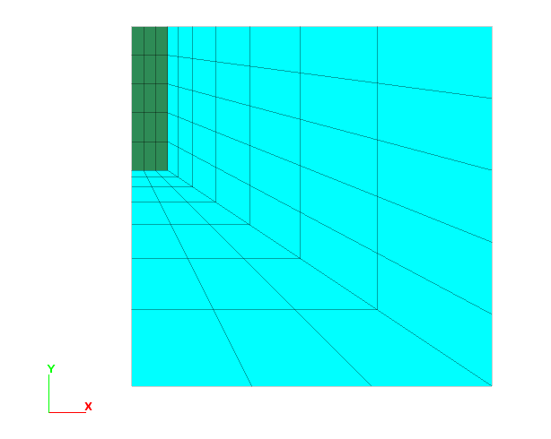
Figure 1: Half-symmetry model of trench excavation.
By default, the boundaries in FLAC2D are free of stress and are unconstrained. Forces or stresses may be applied to any boundary, or portion of a boundary, by means of the zone apply or zone face apply command. Individual components of the stress tensor may be specified. For example, a constant, compressive \(xx\)-stress component of 10 MPa can be applied to a boundary located at \(x\) = 10 with the command
zone face apply stress-xx -10e6 range position-x 10
Remember that compressive stresses are negative. The range keyword is used at the end of the command line to specify the range of action for the zone face apply command shown here. In this case, the boundary condition applies to any boundary faces that fall within the default tolerance (1e-7) of \(x\) = 10. A linearly varying \(xx\)-stress component can be applied with the gradient keyword. For example,
zone face apply stress-xx -20e6 gradient (0,20e5) ...
                range position-x 0 position-y 0 10
With this command, a \(xx\)-stress component is applied to boundary faces located at \(x\) = 0. The \(xx\)-stress varies linearly with \(y\) from \(σ-{xx}\) = 0 at \(y\) = 10, to \(σ-{xx}\) = −20 × 106 at \(y\) = 0.
When gradient is used, a value varies according to the relation
in which \(S\)o is the value at the global coordinate origin
at (\(x\) = 0, \(y\) = 0) and is the value immediately following the stress-xx
keyword, and \(gx\) and \(gy\) specify the variation of the value in the
\(x\)- and \(y\)-directions and are the two numbers following the
gradient keyword.
Note
*Velocity has units of displacement per cycle or step for the static solution mode and displacement per unit time for the dynamic mode.
Displacements cannot be controlled directly in FLAC2D. In fact, they play no part in the calculation process. In order to apply a given displacement to a boundary, it is necessary to prescribe the boundary’s velocity for a given number of steps. If the desired displacement is \(D\), a velocity \(V\) over \(N\) steps (where \(N\) = \(D/V\)) may be applied.* In practice, \(V\) should be kept small and \(N\) large in order to minimize shocks to the system being modeled. The zone face apply command can be used to specify the velocities; gradients may also be specified.
In addition to gradient, the keywords add, multiply, and vary are available for use to modify the values of zone apply and zone face apply commands (and others).
The following command shows how to fix the \(x\)-displacement to zero along a boundary located at \(x\) = 0:
zone face apply velocity-x 0 range position-x 0
This, in effect, creates a roller boundary at which the boundary plane is fixed in the \(x\)-direction, but free to move in the \(y\)-direction.
A pinned boundary condition (i.e., constrained in the \(x\)- and \(y\)-directions) can be specified with the command
zone face apply velocity (0,0) range position-x 0
For real boundaries, the choice of stress or displacement boundary conditions is usually clear. However, for artificial boundaries, such as planes of truncation, either type may be selected. As shown above, a symmetry boundary is always fixed perpendicular to the symmetry plane.
Experience has shown that, generally:
a fixed boundary causes both stresses and displacements to be underestimated;
a stress boundary causes both stresses and displacements to be overestimated; and
the two types of boundary conditions bracket the true solution, so that it is possible to do tests with both boundaries and get a reasonable estimate of the true solution by averaging the two results.
Discussion: Specify Initial Conditions
In this problem, the initial stress state is subjected to gravitational loading. This is added with the model gravity command.
For this problem, all stresses (\(\sigma-{xx}\), \(\sigma-{yy}\), and \(\sigma-{zz}\)) are initialized with the single command zone initialize-stresses. It is possible to supply a separate stress for each component as well (cf. zone initialize stress xx).
Unlike the boundary condition commands, the initial condition commands assign initial values to selected variables; these can change while the computation proceeds. For example, in geological materials, there is an in-situ state of stress in the ground before any excavation or construction is started. By setting the initial conditions in a FLAC2D grid, an attempt is made to reproduce this in-situ state because it will influence the subsequent behavior of the model. (This influence is discussed in more detail in the Boundary Conditions topic.)
To prescribe an initial stress state, the zone initialize command is used. For example,
zone initialize stress xx -50e6 yy -40e6 zz -10e6
This assigns initial compressive stress components of
\(\sigma-{xx}\) = −50e6 |
\(\sigma-{yy}\) = −40e6 |
\(\sigma-{zz}\) = −10e6 |
to all zones in the model. All four stress components (\(xx\), \(yy\), \(zz\), \(xy\)) can be initialized (either individually or all together in one command), and a stress gradient can be specified for boundary stresses in the same manner as previously discussed in Boundary Condition Types (see also Value Modifiers (add, multiply, gradient, & vary keywords) for usage).
If the initial stress state is subjected to gravitational loading, this may be added via the model gravity command. For example,
model gravity (0,-9.81,0)
in which a gravitational acceleration vector of 9.81 m/sec2 is applied in the negative \(y\)-direction. If gravitational loading is specified, the material mass density must also be initialized with the command zone property density.
In the example in this tutorial, \(σ-{xx}\) stresses and gradients are equal to half the \(σ-{yy}\) stresses and gradients. Stresses may be initialized to any value, but one must check the stress state to ensure that it does not violate the yield criterion (Mohr-Coulomb, in this case). The initial equilibrium state is discussed further in the next section.
Step to Equilibrium
Next a series of commands is added to complete the initial model definition.
Type or copy-paste the lines below into the “tutorial” data file.
; Histories
model history mechanical ratio

; step to equilibrium
model large-strain on
model solve
model save 'initial'
Rerun the model to this point by pressing solve (
).Make a new plot by clicking the drop-down menu at the top of the workspace and selecting . Name the plot “ratio”.
Press the Build Plot button (
 ) in the Tools area on the right, and double-click “History Chart”.
In the “Attributes” section, press the plus button (
 ) adjacent to the label “mechanical ratio limit”.
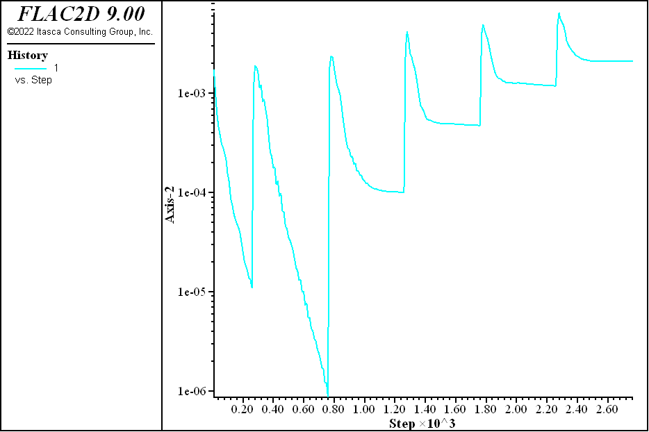
In the attributes for the History item, open the “Axis-2” group (press the arrow adjacent to the label) and check the “Log” box to set the \(y\)-axis of the plot to a logarithmic scale.
Discussion: Stepping to Equilibrium
The FLAC2D model must be at an initial force-equilibrium state before alterations can be performed. For simple model geometries, the boundary conditions and initial conditions may be assigned such that the model is exactly at equilibrium initially. However, in most cases, it is necessary to step the model to the initial equilibrium state under the given boundary and initial conditions, particularly for problems with complex geometries or multiple materials. This is done using either the model step command (or its synonym model cycle) or the model solve command.
In this example, before the model solve command is issued, the program is set to use large-strain calculation, which will move the position of the zones as displacements develop. Also, a history of average convergence ratio is set to be recorded when the model cycles. The history will be used as a means of visualizing and verifying that the model reaches equilibrium.
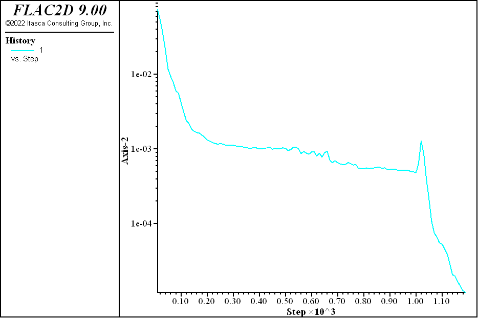
The model will cycle for 1198 steps when the model solve command is given. When complete, this is another juncture where saving the model state is advisable; the last command in the listing above does this.
To verify the model has reached equilibrium, a plot of the convergence ratio is created (steps (3)-(6) above do this). The resulting image should match the one below. The plot indicates that a ratio of 1e-5 is reached after 1198 steps.
Meaning of Equilibrium
A model is in perfect equilibrium when the net nodal-force vector at each gridpoint is zero (see Theoretical Background and following). The convergence criteria used is monitored in FLAC2D and printed to the screen when the model solve command is executing. In this way, the user can assess when equilibrium has been reached.
For a numerical analysis, the average force ratio will never reach exactly zero. It is sufficient, though, to say the model is in equilibrium when it reaches a small value. The default limit of 1e-5 is considered adequate in the majority of cases.
This is an important aspect of numerical problem-solving with FLAC2D. The user must decide when the model has reached equilibrium.
There are several features built into FLAC2D to assist in making this decision. As shown above, recording a history of unbalanced force ratio can be informative. It is also possible to record a history of the maximum unbalanced force by adding the command
model history mechanical unbalanced-maximum
Additionally, the history of selected variables (e.g., velocity or displacement at a gridpoint) may be recorded. The following commands are examples:
zone history velocity-x position (3,4)
zone history displacement-y position (0,8)
The first history command records \(x\)-velocity at location (\(x\) = 3, \(y\) = 4), while the second records \(y\)-displacement at location (\(x\) = 0, \(y\) = 8).
After running several hundred (or thousand) calculation steps, a history of these records may be plotted to indicate the equilibrium condition. The simple example below illustrates this process.
model new
model large-strain off
zone create quadrilateral
model history mechanical unbalanced-maximum
model history mechanical ratio
zone history velocity-x position (3,4)
zone history displacement-y position (0,8)
zone cmodel assign elastic
zone property bulk 3e8 shear 2e8 density 1000
model gravity 10
zone face apply velocity (0,0) range position-y 0
model solve
model solve ratio 1e-6
model solve convergence 1
model step 1500
The initial average force ratio is about 0.24. After 100 steps, this force has dropped to approximately .01. By plotting the first history, it can be seen that the average force ratio is approaching zero. This can be done by creating a plot, adding a “History” plot item, and selecting the mechanical ratio limit history in the Attribute panel. (Note the same plot was made above and changed the \(y\)-axis to logarithmic, which makes it easier to observe the small ratios).
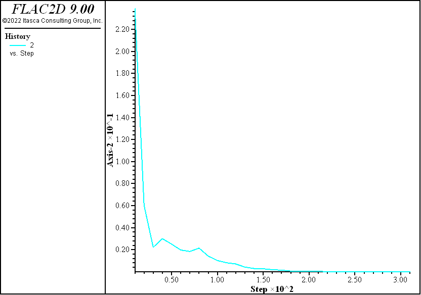
Figure 2: Unbalanced force ratio history.
The velocity also approaches zero, and the displacement history becomes constant; these are indicators that an equilibrium state is reached.
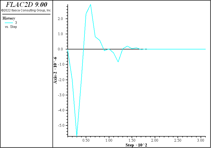
Figure 3: \(x\)-velocity history at (x = 3, z = 4).
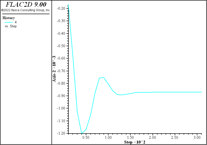
Figure 4: \(y\)-displacement history at (x = 0, y = 8).
By default, an average force ratio limit of 1.0 × 10⁻⁵ is used if no other limits are specified in a model solve. The ratio can be changed by typing
model solve ratio 1e-6
before giving the model solve command. Here 1e-6 is a user-supplied value that sets the limit of the current convergence ratio.
A more robust way of ensuring the model is at equilibrium is to use the following command instead.
model solve convergence 1
Using this approach ensures that every gridpoint has a force ratio below some threshold, rather than ensuring the average force ratio across the entire model is within the bounds. This is useful for large models with small areas of instability that may be masked when looking at the average model unbalanced force ratio. For more information about different convergence criteria refer to Reaching Equilibrium.
It is also possible to bypass the convergence criteria and specify a number of steps. This is useful in the case where a model may not reach equilibrium. The syntax for this would be as shown below.
model step 1500
In the tutorial example, CS: is this the quickstart tutorial?? the initial equilibrium stage was achieved quickly by inserting a zone initialize stress command before the model solve command:
zone initialize-stresses ratio 0.5
This causes the forces to be nearly balanced at the start; the model solves in 267 steps. The forces are not perfectly balanced at the start because of the graded mesh. If zones are all of equal size, the unbalanced force would be nearly zero. However, with graded meshes, it is usually necessary to perform some stepping to bring the model to an initial equilibrium state.
Try commenting out this line (;) and rerunning the tutorial example—it takes nearly twice as many steps to reach equilibrium.
In an analysis, it is very important that the model be at equilibrium before alterations are made. Several histories should be recorded throughout a model to ensure that a large force imbalance does not exist. Analyses are not adversely affected if more steps than needed are taken to reach equilibrium. However, the analysis will be affected if too few steps are taken.
A FLAC2D calculation can be interrupted at any time during stepping by pressing Shift+Esc, or by clicking on the Stop button in the toolbar  . It can be convenient to use the
 model step command with a high step-number to periodically interrupt the stepping, check the histories, and resume stepping until the equilibrium condition is reached.
In the Interface
When cycling, there are some aspects of program operation that are worth noting.
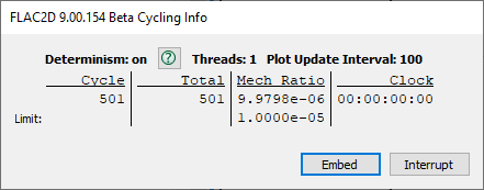
Figure 5: The “Cycling Info” dialog.
The Cycling Info dialog displays a running total of the number of steps in the current step/cycle/solve command, the total number of cycles in the model, the average stress ratio, and the clock time for the current
step/cycle/solvecommand.The current cycling may be interrupted by pressing the button or by pressing the Shift + Esc key.
With regard to the tutorial, note the most recent saved state, “initial.sav”, is added to the “Saved States” list in the Project tile (and it is the active state).
Here and anywhere else it is encountered in FLAC2D, a Help button (
 ) will open a help file topic that provides contextual information for the current item.
Alter Model: Excavation
Now the model excavations are performed.
Type or copy-paste the lines below into the “tutorial” data file.
; excavation step 1
zone cmodel assign null range group "exc1"
model step 500
model save "exc1"
; excavation step 2
zone cmodel assign null range group "exc2"
model step 500
model save "exc2"
; excavation step 3
zone cmodel assign null range group "exc3"
model step 500
model save "exc3"
; excavation step 4
zone cmodel assign null range group "exc4"
model step 500
model save "exc4"
; excavation step 5
zone cmodel assign null range group "exc5"
model step 500
model save "exc5"

; install cable support
model restore "exc2"
Rerun the model to this point by pressing solve (
).Make the “History” plot tile active.
Discussion: Performing Alterations
Before performing the excavations, a couple of additional histories are set up—one for \(x\)-displacement at the gridpoint at (-1,-0.01) (top, left of the trench), and one for \(y\)-displacement at the same location. Note that for the top point, a location slightly below \(y\) = was specified. This is because the model is run in large strain mode, so the top of the model moves down slightly and specifying a coordinate of (-1,0) would fall outside of the model.
Excavation is a matter of first assigning the zones of the current excavation stage to the null model. The model is then cycled for 500 steps, and then the model state is saved before moving on to the next excavation stage. Note the zone groups for the excavation stages that were created in Create Model Groups are used for the zone cmodel assign commands that perform the excavation.
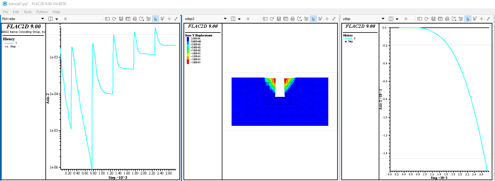
The “History” plot shows that the five excavation stages have been added to the history seen in the previous step (one + five minimum points in the chart are seen). Significantly, failure in the third stage is observed—it does not reach/approach a convergence ratio of 1e-5 before the next excavation step begins.
At this point, it should be observed that the use of the model step command in this example is a bit unrealistic. It is used here to help illustrate the modeling process efficiently. However, in a more rigorous model, the command model solve would be used, and the failure in the third step would be evident—the model would simply continue to cycle. Test this by substituting model solve for model step 500 at the third excavation stage. The model will eventually stop cycling, but with an “Illegal geometry” error; it never reaches equilibrium. This is a common terminating point on models exhibiting continuous deformation. It indicates a zone deformation in the model too extreme to allow further calculations on it.
The next modeling phase of this tutorial will involve installing cables as support after the second stage and observing the effect. However, before doing so, plotting is reexamined to get a further look at the failure that occurs in the third stage.
Further Discussion: Performing Alterations
FLAC2D allows model conditions to be changed at any point in the solution process. These changes may take the following forms:
excavation of material;
addition or deletion of gridpoint loads or stresses;
change of material model or properties for any zone; and
fix or free velocities for any gridpoint.
Note
*If moduli (bulk or shear) are changed in a model that is in equilibrium, no immediate effect will be observed because FLAC2D uses tangent, rather than secant, moduli.
In this tutorial, excavation is performed using the zone cmodel assign null command. Gridpoint loads can be applied at any gridpoint with the zone apply (force, force-x, etc.) command. Stress alterations can be made at model boundaries with the zone face apply command, as shown previously. Material models and properties* are changed with the zone cmodel assign and zone property commands. Gridpoint velocities are fixed or freed using the zone face apply command to set velocity to the desired value(s). It should be evident that several commands can be repeated to perform various model alterations.
If model zones contain a plasticity model (e.g., zone cmodel assign mohr-coulomb), it is possible that an alteration may be such that force equilibrium cannot be achieved. In other words, the unbalanced forces in part or all of the model cannot approach zero, in which case the average force ratio will approach a constant nonzero value, indicating that steady-state flow of material is occurring (i.e., a portion/all of the model is failing).
Examine Model: Plotting
The following steps illustrate the basic mechanics of plotting.
From the drop-down menu at the top of the workspace select and name it “xdisp” in the ensuing dialog. Note the newly created empty plot is now active in the Workspace. (Alternatively, create a plot from the main menu: .)
Press the Build Plot button (
), select History Chart and press in the ensuing dialog.In the “Attributes” section on the Control Panel:
add History 2 “X Displacement at …” by pressing the add button adjacent to its label (
);open the “X-axis” item, uncheck “Auto” on “Minimum” and “Maximum”, and type “0” in for the minimum and “2800” in for the maximum; and
open the “Y-axis” item, uncheck “Auto” on “Maximum”, and type in the “0.1” for the maximum value.
Repeat steps 1-2 to create a History plot of \(y\)-displacement named “ydisp”.
In the “ydisp” plot, go to the “Attributes” section:
add History 3 “Y Displacement at …” by pressing the add button adjacent to its label (
);open the “X-axis” item, uncheck “Auto” on “Minimum” and “Maximum”, and type “0” in for the minimum and “2800” in for the maximum; and
open the “Y-axis” item, uncheck “Auto” on “Minimum”, and type in the “-0.16” for the minimum value.
Press Ctrl + Shift + N, and name the new plot “xdisp2”.
Press the Build Plot button (
), select Zone and press in the ensuing dialog.In the “Attributes” control set:
select “Contour” on the “Color By” switch;
select “Displacement” on the “Value” switch;
select “Y” on the “Component” switch;
open the “Contour” item, and check the “Reversed” box; and
uncheck “Auto” on “Minimum,” and set the value of the minimum to “-0.16”.
Now, with any of these three plots active, step through the saved model states in the Project panel by double-clicking each saved state. Start with the “initial” state (initial equilibrium), then progress through the excavation stages (“exc1” through “exc5”).
Discussion: Observing Failure
The failure as the excavation sequence progresses is observed by plotting the history items that were defined prior to running the model (immediately after initial equilibrium had been established). History plots, by default, automatically compute the maximum and minimum values for the scales on the \(x\)- and \(y\)-axis of the chart. This is efficient and time-saving when looking at that history at a single model state. However, when looking at the same thing across a series of model states, it makes comparison of one view to the next difficult, because the scale on either axis is likely to change from one state to the next. For this reason, when setting up the plots here to help visualize the failure that occurs starting in the third excavation stage, the scales on the plots are “fix”ed by turning the “Auto” attribute off. As a result, when stepping through the saved states (step (9) above), the fixed scales allow clear observation of the developing failure without any “jumping around” in the chart.
Plots As Project Entities
Unlike command input or model states, plots are not stored separately as files. Once created, they will be saved with the project. Closing a plot ( ![]() ) hides it from view, but it can be recovered by double-clicking on the plot name in the Project panel.
) hides it from view, but it can be recovered by double-clicking on the plot name in the Project panel.
Four reference plots are named. When creating a new plot, FLAC2D automatically suggests a numbered name (e.g., “Plot04”), but as can be seen here, providing a more descriptive name is helpful, especially when many plots have been created. To change a plot name after it has been created, right-click on the plot name in the Project panel and select :menuselection:` Rename Plot …`.
The Workspace may be split to show more than one plot simultaneously. Click on the split button ( ![]() ) adjacent to the content selector to do this. Use the content selector to load each plot as desired. Click and drag on the bars between the plots to resize them.
) adjacent to the content selector to do this. Use the content selector to load each plot as desired. Click and drag on the bars between the plots to resize them.
In the Interface
The basic mechanics of model visualization in the Model view or in a plot in the Workspace are as follows.
Put objects into the view. In the Model pane, this occurs automatically as model objects (zones, structural elements) are created. In a Plot, this is done by picking items from the Build Plot dialog using the Build Plot tool (
).The objects that are currently rendered in the view are listed above in the Control Panel.
To control how an object is rendered, select it on the list above. This will activate the controls for visualization that appear below—for that object—in the “Attributes” section.
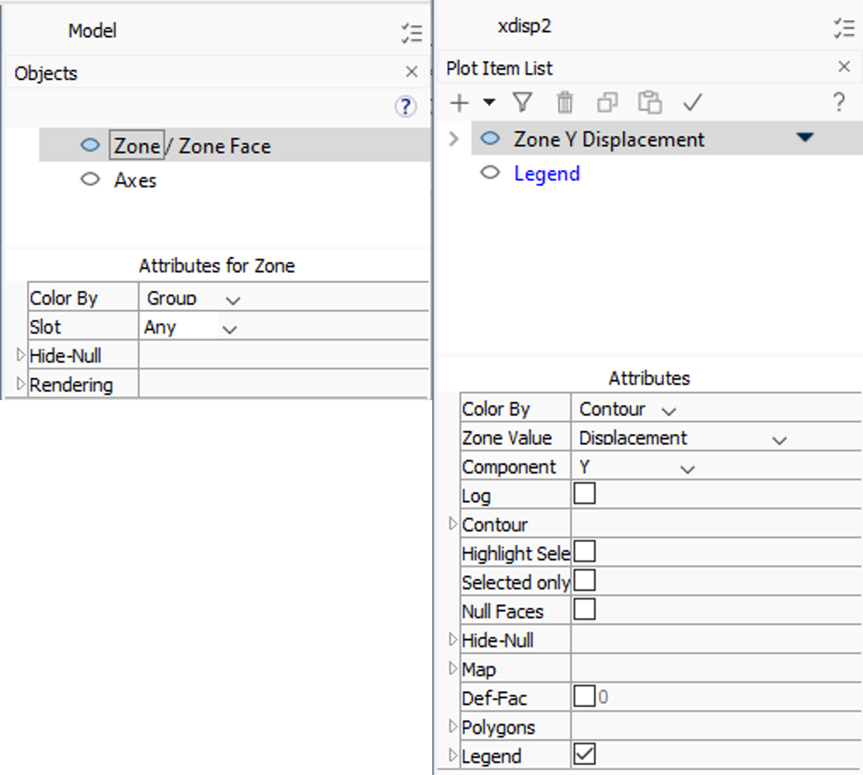
Figure 6: Two views of the Tools panel: the “Objects” control set in the Model pane (left), and the “Plot Item List” in a Plot.
In the Model view, Zones and Zone Faces are listed on the same line of the “Objects” control set. Only one may be rendered at a time. A box indicates which is currently being rendered. Clicking the other item’s label will cause it to be rendered instead.
Selecting a plot item in a Plot causes a menu selector icon (
 ) to appear to the right of the item name. The menu provides options to set attributes, add a plot item, or to cut, copy, delete, or paste the current item.
Further Alterations: Support
Support is installed after the second excavation stage to stabilize the trench and prevent the failure seen in the third excavation stage.
Type or copy-paste the lines below into the “tutorial” data file.
; install cable support
model restore "exc2"
structure cable create ...
            by-ray (1.0,0.4,1.5) (1,0,0) 4 segments 4
structure cable create ...
            by-ray (1.0,0.4,0.5) (1,0,0) 4 segments 4
structure cable create ...
            by-ray (1.0,1.2,1.5) (1,0,0) 4 segments 4
structure cable create ...
            by-ray (1.0,1.2,0.5) (1,0,0) 4 segments 4
structure cable property young 2e9 ...
            yield-tension 1e8 ...
            cross-sectional-area 1.0 ...
            grout-cohesion 1e10 ...
            grout-stiffness 2e9 ...
            grout-perimeter 1.0
zone cmodel assign null range group "exc3"
model step 500
model save "cab3"
structure cable create ...
            by-ray (1.0,2.0,1.5) (1,0,0) 4 segments 4
structure cable create ...
            by-ray (1.0,2.0,0.5) (1,0,0) 4 segments 4
structure cable property young 2e9 ...
            yield-tension 1e8 ...
            cross-sectional-area 1.0 ...
            grout-cohesion 1e10 ...
            grout-stiffness 2e9 ...
            grout-perimeter 1.0
zone cmodel assign null range group "exc4"
model step 500
model save "cab4"
structure cable create ...
            by-ray (1.0,2.8,1.5) (1,0,0) 4 segments 4
structure cable create ...
            by-ray (1.0,2.8,0.5) (1,0,0) 4 segments 4
structure cable property young 2e9 ...
            yield-tension 1e8 ...
            cross-sectional-area 1.0 ...
            grout-cohesion 1e10 ...
            grout-stiffness 2e9 ...
            grout-perimeter 1.0
zone cmodel assign null range group "exc5"
model step 500
model save "cab5"
Rerun the model to this point by pressing solve (
).
Discussion: Installing Cables
Using the model restore command, the model state after two excavation stages — while it is still stable — is reestablished. Now support is added in addition to nulling the zones for each excavation stage. This is done by spatially defining the cable, and then defining its properties. Then (as before) the excavation stage zones are nulled, the model is cycled 500 steps, and the model state is saved. This sequence is repeated to create a new third, fourth, and fifth excavation stage.
Further Discussion: Using Save/Restore and Staged Modeling
At this point, the function of the commands model save and model restore in a staged analysis should be apparent. At the end of a modeling stage (e.g., initial equilibrium), the model state can and should be saved using model save. This file can be restored at a later time using model restore, which will put the model back to the point at which the model was saved. Consequently, it is not necessary to build a model from scratch every time a change is made; simply save the model before the change and restore it to that point whenever a new change is to be analyzed.
For example, in this tutorial trench problem, the trench is excavated in 2 m deep stages. The model state is saved at the end of each stage, beginning with the initial equilibrium stage (“initial”). Looking at each stage in sequence helps determine the stage at which the trench fails, which then suggests investigating the influence of support (e.g., tiebacks or soil nails) on stabilizing the trench.
Determining, upon running the model, that the trench fails at the third excavation stage, the save file at the second excavation stage (exc2.sav) is restarted, cables are installed, and then excavation proceeds. This time, the trench walls are stable.
Using save files this way allows a series of different calculations that start from any desired stage to investigate various problem conditions, such as spacing and properties of cable elements.
In the Interface
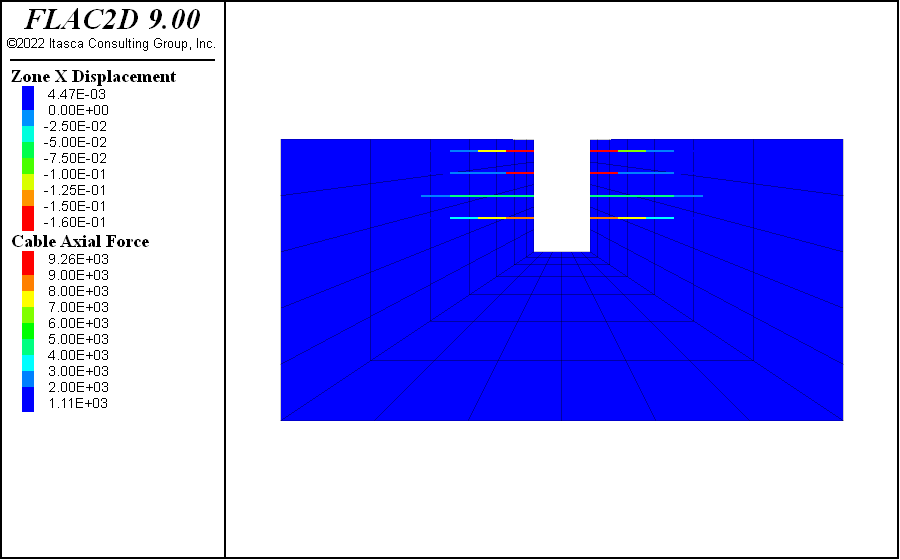
Make the “xdisp2” plot active. Click the Build Plot button (![]() ) and select Cable from the list. By default the cables will be colored by group. Change Color By to Contour and Value to Axial Force. The cables and the forces generated are now visible. Notice that the \(x\)-displacement in the zones is small since the cables are supporting the trench (recall the maximum contour is fixed to a large value, so all of the zones appear blue).
) and select Cable from the list. By default the cables will be colored by group. Change Color By to Contour and Value to Axial Force. The cables and the forces generated are now visible. Notice that the \(x\)-displacement in the zones is small since the cables are supporting the trench (recall the maximum contour is fixed to a large value, so all of the zones appear blue).
Project Finishing
The project is complete at this point. For the purpose of good management, a few additional steps are advisable.
Use to save the current project.
Bundle the project by selecting the menu command
In the ensuing dialog, review the contents to be packed, press , and provide a name for the bundle file.
Discussion: Project Completion
With the model runs completed, the project is saved and, for good measure, a bundle file is created for the project.
At this point, the modeling process should be clearer. This tutorial illustrates that model setup and specification of initial definitions tend to follow a singular path, However, once past the equilibrium stage, the potential for branching and bifurcation due to exploration, revision, and alteration is nearly limitless. In that context, a well-designed project with distinct stages is critically important.
About Bundles
A bundle is a compressed archive file that gathers up the following:
any files input in the model (the files listed in the “Data Files” section of the Project panel);
state record files (a record file corresponding to each save file listed in the “Saved States” section of the Project tile); and
the project file.
With a bundle file, all materials necessary to re-create the project are stored in a single location. Because the bundle file does not store save files—which can be quite sizable when a model is large—it is a useful, efficient way to archive a project. The trade-off for that efficiency, however, is that using a bundle to re-create a project will require re-running the component data files or replaying the state record files in order to regenerate the project saved state(s).
Bundles are also an excellent way of attaching the project to a technical support request. This can be done automatically when requesting technical support via the technical support dialog ().
In the Interface: Finishing
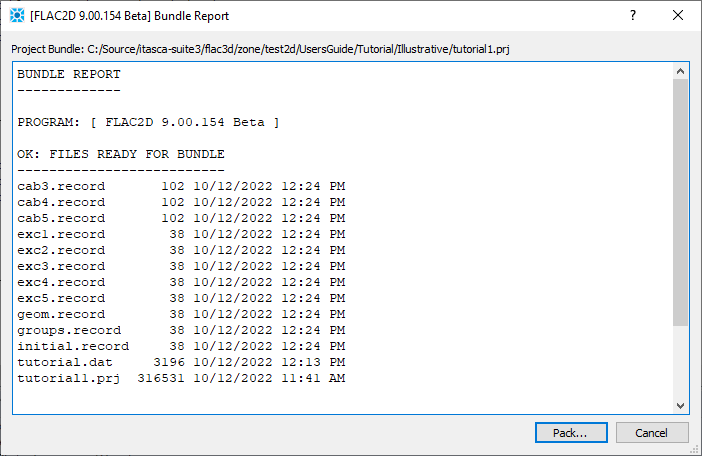
The bundle file report “previews” the content that will be included in the bundle.
There should be a .record file corresponding to each .sav file in the project.
The project file and all input files (data files, etc.) are included in the bundle.
The file report categorizes the bundle contents in different sections: “OK”, “Warning: Files Modified But Not Saved”, “Error: Files Cannot Be Located (Link Broken)”, etc. For this tutorial, which is comparatively simple, all content is “OK”. Refer to the Bundle Report topic for reference.
Endnotes
| Was this helpful? ... | Itasca Software © 2024, Itasca | Updated: Nov 12, 2025 |
